Overview
- R objects
- Data structures and types
- Indexing and subsetting
- Attributes
- Factors
R objects
Everything is an object.
John Chambers
- Fundamentally, everything you are dealing with in R is an object
- That includes individual variables, datasets, functions and many other classes of objects
- The key reference to an object is its name
- Typically, the reference is established through assignment operation
Assignment operations
<-is the standard assignment operator in R- While
=is also supported it is not recommended - As it hides the difference between
<-and<<-(deep assignment)
In [2]:
x <- 3
x
[1] 3
In [3]:
x <- 3
f <- function() {
    x <<- 1 # Modifies the existing variable in parent namespace (or creates a new global variable)
}
f()
x
[1] 1
Membership operations
Operator %in% returns TRUE if an object of the left side is in a sequence on the right.
In [4]:
"a" %in% "abc" # Note that R strings are not sequences
[1] FALSE
In [5]:
3 %in% c(1, 2, 3) # c(1, 2, 3) is a vector
[1] TRUE
In [6]:
!(3 %in% c(1, 2, 3))
[1] FALSE
Data structures
Base R data structures can be classified along their dimensionality and homogeneity
5 main built-in data structures in R:
- Atomic vector (
vector) - Matrix (
matrix) - Array (
array) - List (
list) - Data frame (
data.frame)
Summary of data structures in R
| Structure | Description | Dimensionality | Data Type |
|---|---|---|---|
vector |
Atomic vector (scalar) | 1d | homogenous |
matrix |
Matrix | 2d | homogenous |
array |
One-, two or n-dimensional array | 1d/2d/nd | homogenous |
list |
List | 1d | heterogeneous |
data.frame |
Rectangular data | 2d | heterogeneous |
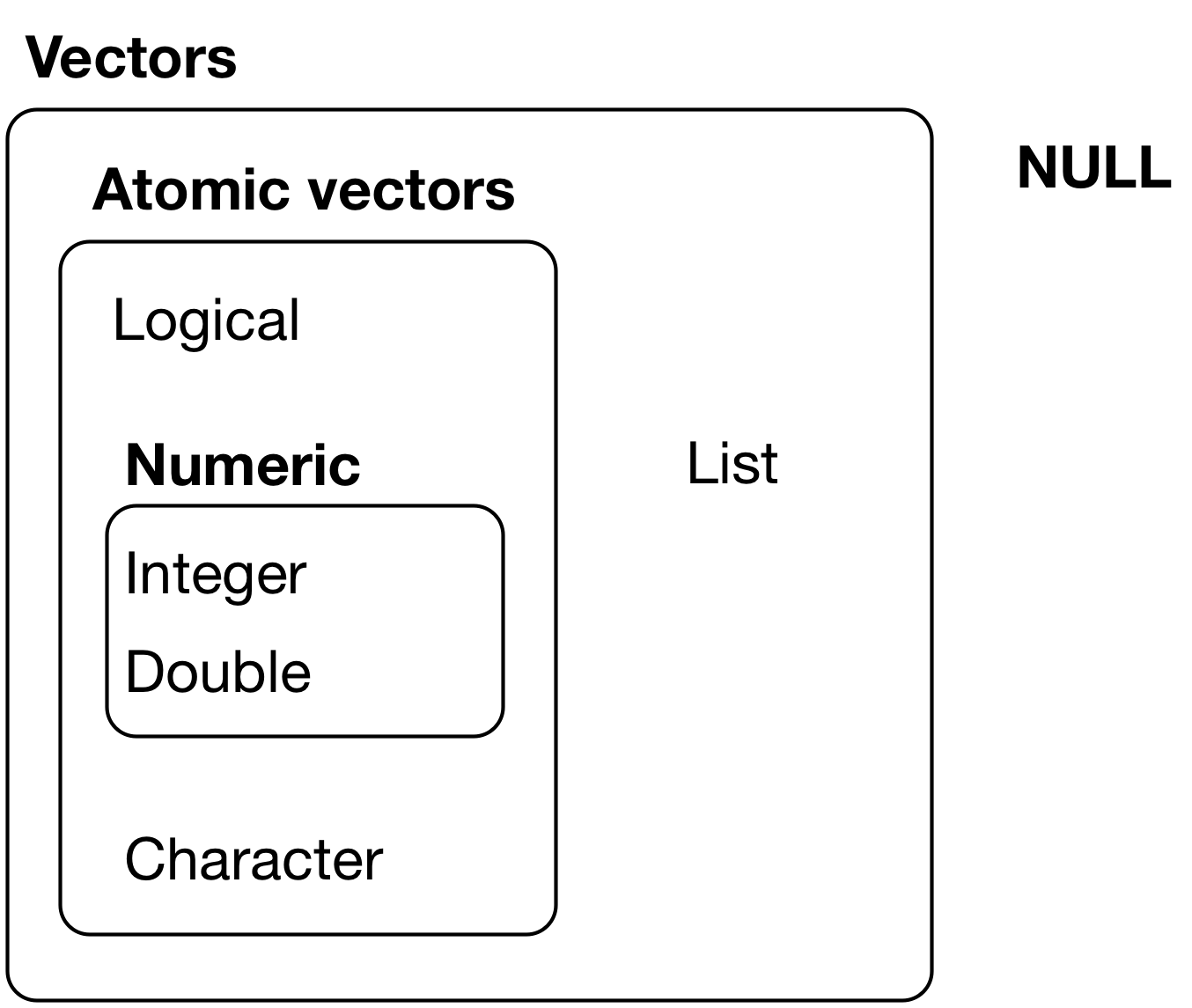
Atomic vectors
- Vector is the core building block of R
- R has no scalars (they are just vectors of length 1)
- Vectors can be created with
c()function (short for combine)
In [7]:
v <- c(8, 10, 12)
v
[1] 8 10 12
In [8]:
v <- c(v, 14) # Vectors are always flattened (even when nested)
v
[1] 8 10 12 14
Data types
4 common data types that are contained in R structures:
- Character (
character) - Integer (
integer) - Double/numeric (
double/numeric) - Logical/boolean (
logical)
Character vector
In [9]:
char_vec <- c("apple", "banana", "watermelon")
In [10]:
char_vec
[1] "apple" "banana" "watermelon"
In [11]:
# length() function gives the length of an R object (analogous to Python's len())
length(char_vec)
[1] 3
In [12]:
is.character(char_vec)
[1] TRUE
Integer vector
In [13]:
# Note the 'L' suffix to make sure you get an integer rather than double
int_vec <- c(300L, 200L, 4L)
In [14]:
int_vec
[1] 300 200 4
In [15]:
# typeof() function returns the type of an R object (analogous to Python's type())
typeof(int_vec)
[1] "integer"
In [16]:
# is.integer() tests whether R object (vector/array/matrix) contains elements of type 'integer'
is.integer(int_vec)
[1] TRUE
Double vector
In [17]:
# Note that even without decimal part R treats these numbers as double
dbl_vec <- c(300, 200, 4)
In [18]:
dbl_vec
[1] 300 200 4
In [19]:
typeof(dbl_vec)
[1] "double"
In [20]:
is.double(dbl_vec)
[1] TRUE
In [21]:
# Note that is.numeric() function is a generic way of testing whether vector has numbers:
# integers or double
is.numeric(int_vec)
[1] TRUE
Integer vs double
- Integers are used to store whole numbers (e.g. counts)
- 32-bit integer: $2^{32} = 4,294,967,296$
- Signed 32-bit integer: $[-2,147,483,648 \mathrel{{.}\,{.}} 2,147,483,648]$
Logical vector
In [22]:
log_vec <- c(FALSE, FALSE, TRUE)
log_vec
[1] FALSE FALSE TRUE
In [23]:
# While more concise, using T/F instead of TRUE/FALSE can be confusing
log_vec2 <- c(F, F, T)
log_vec2
[1] FALSE FALSE TRUE
In [24]:
typeof(log_vec)
[1] "logical"
Type coercion in vectors
- All elements of a vector must be of the same type
- If you try to combine vectors of different types, their elements will be coerced to the most flexible type
In [25]:
# Note that logical vector get coerced to 0/1 for FALSE/TRUE
c(dbl_vec, log_vec)
[1] 300 200 4 0 0 1
In [26]:
c(char_vec, int_vec)
[1] "apple"      "banana"     "watermelon" "300"        "200"
[6] "4"
In [27]:
# If no natural way of type conversion exists, NAs are introduced
as.numeric(char_vec)
Warning message in eval(expr, envir, enclos):
“NAs introduced by coercion”
[1] NA NA NA
NA and NULL values
- R makes a distinction between:
NA- value exists, but is unknown (e.g. survey non-response)NULL- object does not exist
NA's are defined for each data type (integer, character, numeric, etc.)
Extra: R Documentation on NA
NA and NULL example
In [28]:
na <- c(NA, NA, NA)
na
[1] NA NA NA
In [29]:
length(na)
[1] 3
In [30]:
null <- c(NULL, NULL, NULL)
null
NULL
In [31]:
length(null)
[1] 0
Working with NAs
In [32]:
# Presence of NAs can lead to unexpected results
v_na <- c(1, 2, 3, NA, 5)
mean(v_na)
[1] NA
In [33]:
# NAs should be treated specially
mean(v_na, na.rm = TRUE)
[1] 2.75
In [34]:
# Remember NAs are missing values
# Thus result of comparing them is unknown
NA == NA
[1] NA
In [35]:
# is.na() is a special function that checks whether value is missing (NA)
is.na(v_na)
[1] FALSE FALSE FALSE TRUE FALSE
In [36]:
# We can use such logical vectors for subsetting (more below)
v_na[!is.na(v_na)]
[1] 1 2 3 5
Vector indexing and subsetting
- Indexing in R starts from 1 (as opposed to 0 in Python)
- To subset a vector, use
[]to index the elements you would like to select:
vector[index]In [37]:
dbl_vec[1]
[1] 300
In [38]:
dbl_vec[c(1,3)]
[1] 300 4
Summary of vector subsetting
| Value | Example | Description |
|---|---|---|
| Positive integers | v[c(3, 1)] |
Returns elements at specified positions |
| Negative integers | v[-c(3, 1)] |
Omits elements at specified positions |
| Logical vectors | v[c(FALSE, TRUE)] |
Returns elements where corresponding logical value is TRUE |
| Character vector | v[c(“c”, “a”)] |
Returns elements with matching names (only for named vectors) |
| Nothing | v[] |
Returns the original vector |
| 0 (Zero) | v[0] |
Returns a zero-length vector |
Generating sequences for subsetting
- You can use
:operator to generate vectors of indices for subsetting seq()function provides a generalization of:for generating arithemtic progressions
In [39]:
2:4
[1] 2 3 4
In [40]:
# It is similar to Python's object[start:stop:step] syntax
seq(from = 1, to = 4, by = 2)
[1] 1 3
Vector subsetting examples
In [41]:
v
[1] 8 10 12 14
In [42]:
v[2:4]
[1] 10 12 14
In [43]:
# Argument names can be omitted for matching by position
v[seq(1,4,2)]
[1] 8 12
In [44]:
# All but the last element
v[-length(v)]
[1] 8 10 12
In [45]:
# Reverse order
v[seq(length(v),1,-1)]
[1] 14 12 10 8
Vector recycling
For operations that require vectors to be of the same length R recycles (reuses) the shorter one
In [46]:
c(0, 1) + c(1, 2, 3, 4)
[1] 1 3 3 5
In [47]:
5 * c(1, 2, 3, 4)
[1] 5 10 15 20
In [48]:
c(1, 2, 3, 4)[c(TRUE, FALSE)]
[1] 1 3
which() function
Returns indices of TRUE elements in a vector
In [49]:
char_vec
[1] "apple" "banana" "watermelon"
In [50]:
char_vec == "watermelon"
[1] FALSE FALSE TRUE
In [51]:
which(char_vec == "watermelon")
[1] 3
In [52]:
dbl_vec[char_vec == "watermelon"]
[1] 4
In [53]:
dbl_vec[which(char_vec == "watermelon")]
[1] 4
Lists
- As opposed to vectors, lists can contain elements of any type
- List can also have nested lists within it
- Lists are constructed using
list()function in R
In [54]:
# We can combine different data types in a list and, optionally, name elements (e.g. B below)
l <- list(2:4, "a", B = c(TRUE, FALSE, FALSE), list("x", 1L))
l
[[1]]
[1] 2 3 4

[[2]]
[1] "a"

$B
[1]  TRUE FALSE FALSE

[[4]]
[[4]][[1]]
[1] "x"

[[4]][[2]]
[1] 1
R object structure
str()- one of the most useful functions in R- It shows the structure of an arbitrary R object
In [55]:
str(l)
List of 4
 $  : int [1:3] 2 3 4
 $  : chr "a"
 $ B: logi [1:3] TRUE FALSE FALSE
 $  :List of 2
  ..$ : chr "x"
  ..$ : int 1
List subsetting
- As with vectors you can use
[]to subset lists - This will return a list of length one
- Components of the list can be individually extracted using
[[and$operators
list[index]
list[[index]]
list$name
List subsetting examples
In [56]:
l[3]
$B
[1]  TRUE FALSE FALSE
In [57]:
str(l[3])
List of 1
 $ B: logi [1:3] TRUE FALSE FALSE
In [58]:
l[[3]]
[1] TRUE FALSE FALSE
In [59]:
# Only works with named elements
l$B
[1] TRUE FALSE FALSE
Attributes
- All R objects can have attributes that contain metadata about them
- Attributes can be thought of as named lists
- Names, dimensions and class are common examples of attributes
- They (and some other) have special functions for getting and setting them
- More generally, attributes can be accessed and modified individually with
attr()function
Attributes examples
In [60]:
v
[1] 8 10 12 14
In [61]:
attr(v, "example_attribute") <- "This is a vector"
In [62]:
attr(v, "example_attribute")
[1] "This is a vector"
In [63]:
# To set names for vector elements we can use names() function
names(v) <- c("a", "b", "c", "d")
v
 a  b  c  d
 8 10 12 14
attr(,"example_attribute")
[1] "This is a vector"
In [64]:
# Names of vector elements can be used for subsetting
v["b"]
 b
10
Factors
- Factors form the basis of categorical data analysis in R
- Values of nominal (categorical) variables represent categories rather than numeric data
- Examples are abundant in social sciences (gender, party, region, etc.)
- Internally, in R factor variables are represented by integer vectors
- With 2 additional attributes:
class()attribute which is set tofactorlevels()attribute which defines allowed values
Factors example
In [65]:
cities <- c("Dublin", "Cork", "Cork", "Limerick", "Galway")
cities
[1] "Dublin" "Cork" "Cork" "Limerick" "Galway"
In [66]:
typeof(cities)
[1] "character"
In [67]:
# We use factor() function to convert character vector into factor
# Only unique elements of character vector are considered as a level
cities <- factor(cities)
cities
[1] Dublin   Cork     Cork     Limerick Galway
Levels: Cork Dublin Galway Limerick
In [68]:
class(cities)
[1] "factor"
In [69]:
# Note that the data type of this vector is integer (and not character)
typeof(cities)
[1] "integer"
Factors example continued
In [70]:
# Note that R automatically sorted the categories alphabetically
levels(cities)
[1] "Cork" "Dublin" "Galway" "Limerick"
In [71]:
# You can change the reference category using relevel() function
cities <- relevel(cities, ref = "Dublin")
levels(cities)
[1] "Dublin" "Cork" "Galway" "Limerick"
In [72]:
# Or define an arbitrary ordering of levels using levels argument in factor() function
cities <- factor(cities, levels = c("Limerick", "Galway", "Dublin", "Cork"))
levels(cities)
[1] "Limerick" "Galway" "Dublin" "Cork"
In [73]:
# Under the hood factors continue to be integer vectors
as.integer(cities)
[1] 3 4 4 1 2
Tabulation
table()function is very useful for describing discrete data.- It can be used for:
- tabulating a single variable
- creating contingency tables (crosstabs).
- Implicitly, R treats tabulated variables as factors.
In [74]:
var_1 <- sample(c("a", "b", "c"), size = 50, replace = TRUE)
var_2 <- sample(c(1, 2, 3), size = 50, replace = TRUE)
In [75]:
table(var_1, var_2)
     var_2
var_1 1 2 3
    a 7 5 5
    b 7 5 9
    c 4 6 2
Factors in crosstabs
In [76]:
var_2 <- factor(var_2, levels = c(3, 1, 2))
In [77]:
table(var_2)
var_2
 3  1  2
16 18 16
In [78]:
var_2 <- factor(var_2, levels = c(3, 1, 2), labels = c("Three", "One", "Two"))
In [79]:
table(var_1, var_2)
     var_2
var_1 Three One Two
    a     5   7   5
    b     9   7   5
    c     2   4   6
Arrays and matrices
- Arrays are vectors with an added class and dimensionality attribute
- These attributes can be accessed using
class()anddim()functions - Arrays can have an arbitrary number of dimensions
- Matrices are special cases of arrays that have just two dimensions
- Arrays and matrices can be created using
array()andmatrix()functions - Or by adding dimension attribute with
dim()function
Array example
In [80]:
# : operator can be used generate vectors of sequential numbers
a <- 1:12
a
[1] 1 2 3 4 5 6 7 8 9 10 11 12
In [81]:
class(a)
[1] "integer"
In [82]:
dim(a) <- c(3, 2, 2)
a
, , 1

     [,1] [,2]
[1,]    1    4
[2,]    2    5
[3,]    3    6

, , 2

     [,1] [,2]
[1,]    7   10
[2,]    8   11
[3,]    9   12
In [83]:
class(a)
[1] "array"
Matrix example
In [84]:
m <- 1:12
In [85]:
dim(m) <- c(3, 4)
m
     [,1] [,2] [,3] [,4]
[1,] 1    4    7    10
[2,] 2    5    8    11
[3,] 3    6    9    12
In [86]:
# Alternatively, we could use matrix() function
m <- matrix(1:12, nrow = 3, ncol = 4)
m
     [,1] [,2] [,3] [,4]
[1,] 1    4    7    10
[2,] 2    5    8    11
[3,] 3    6    9    12
In [87]:
# Note that length() function displays the length of underlying vector
length(m)
[1] 12
Array and matrix subsetting
- Subsetting higher-dimensional (> 1) structures is a generalisation of vector subsetting
- But, since they are built upon vectors there is a nuance (albeit uncommon)
- They are usually subset in 2 ways:
- with multiple vectors, where each vector is a sequence of elements in that dimension
- with 1 vector, in which case subsetting happens from the underlying vector
array[vector_1, vector_2, ..., vector_n]
array[vector]
Array subsetting example
In [88]:
a
, , 1

     [,1] [,2]
[1,]    1    4
[2,]    2    5
[3,]    3    6

, , 2

     [,1] [,2]
[1,]    7   10
[2,]    8   11
[3,]    9   12
In [89]:
# Most common way
a[1, 2, 2]
[1] 10
In [90]:
# Specifying drop = FALSE after indices retains the original dimensionality of matrix/array
a[1, 2, 2, drop = FALSE]
, , 1

     [,1]
[1,]   10
In [91]:
# Here elements are subset from underlying vector (with repetition)
a[c(1, 2, 2)]
[1] 1 2 2
Matrix subsetting example
In [92]:
m
     [,1] [,2] [,3] [,4]
[1,] 1    4    7    10
[2,] 2    5    8    11
[3,] 3    6    9    12
In [93]:
# As with arrays drop = FALSE prevents from this object being collapsed into 1-dimensional vector
m[, 1, drop = FALSE]
     [,1]
[1,] 1
[2,] 2
[3,] 3
In [94]:
# Subset all rows, first two columns
m[1:nrow(m), 1:2]
     [,1] [,2]
[1,] 1    4
[2,] 2    5
[3,] 3    6
In [95]:
# Note that vector recycling also applies here
m[c(TRUE, FALSE), -3]
     [,1] [,2] [,3]
[1,] 1    4    10
[2,] 3    6    12
Naming conventions
- Even while allowed in R, do not use
.in variable names (it works as an object attribute in Python) - Do not name give objects the names of existing functions and variables (e.g.
c,T,list,mean) - Use UPPER_CASE_WITH_UNDERSCORE for named constants (e.g. variables that remain fixed and unmodified)
- Use lower_case_with_underscores for function and variable names
Code layout
- Limit all lines to a maximum of 79 characters.
- Break up longer lines
my_long_vector <- c(
  1, 2, 3, 4, 5, 6, 7, 8, 9, 10, 11, 12, 13, 14, 15, 16, 17, 18, 19, 20, 21, 22,
  23, 24, 25, 26, 27, 28, 29, 30, 31, 32, 33, 34, 35, 36, 37, 38, 39, 40, 41,
  42, 43, 44, 45, 46, 47, 48, 49, 50, 51, 52, 53, 54, 55, 56, 57, 58, 59, 60
)

long_function_name <- function(a = "a long argument",
                               b = "another argument",
                               c = "another long argument") {
  # As usual code is indented by two spaces.
}
Reserved words
There are 14 (plus some variations of them) reserved words in R that cannot be used as identifiers.
break |
NA |
else |
NaN |
FALSE |
next |
for |
NULL |
function |
repeat |
if |
TRUE |
Inf |
while |
Source: R reserved words
R packages
- R's flexibility comes from its rich package ecosystem
- Comprehensive R Archive Network (CRAN) is the official repository of R packages
- At the moment it contains > 18K external packages
- Use
install.packages(<package_name>)function to install packages that were released on CRAN - Check
devtoolspackage if you need to install a package from other sources (e.g. GitHub, Bitbucket, etc.) - Type
library(<package_name>)to load installed packages
Help!
R has an inbuilt help facility which provides more information about any function:
In [96]:
?length
In [97]:
help(dim)
- The quality of documentation varies a lot across packages.
- Stackoverflow is a good resource for many standard tasks.
- For custom packages it is often helpful to check the issues page on the GitHub.
- E.g. for
ggplot2: https://github.com/tidyverse/ggplot2/issues - Or, indeed, any search engine #LMDDGTFY
Next
- Control flow and functions