Overview
- Conditional statements
- Loops and Iteration
- Function definition and function call
- Functionals
- Scoping in R
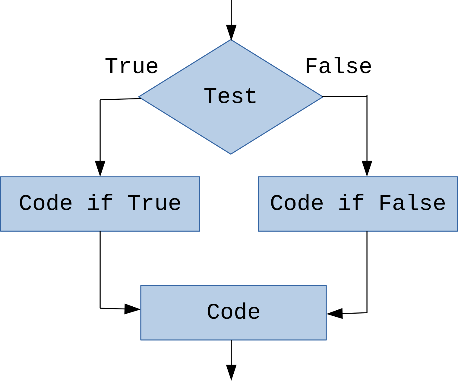
Algorithm flowchart
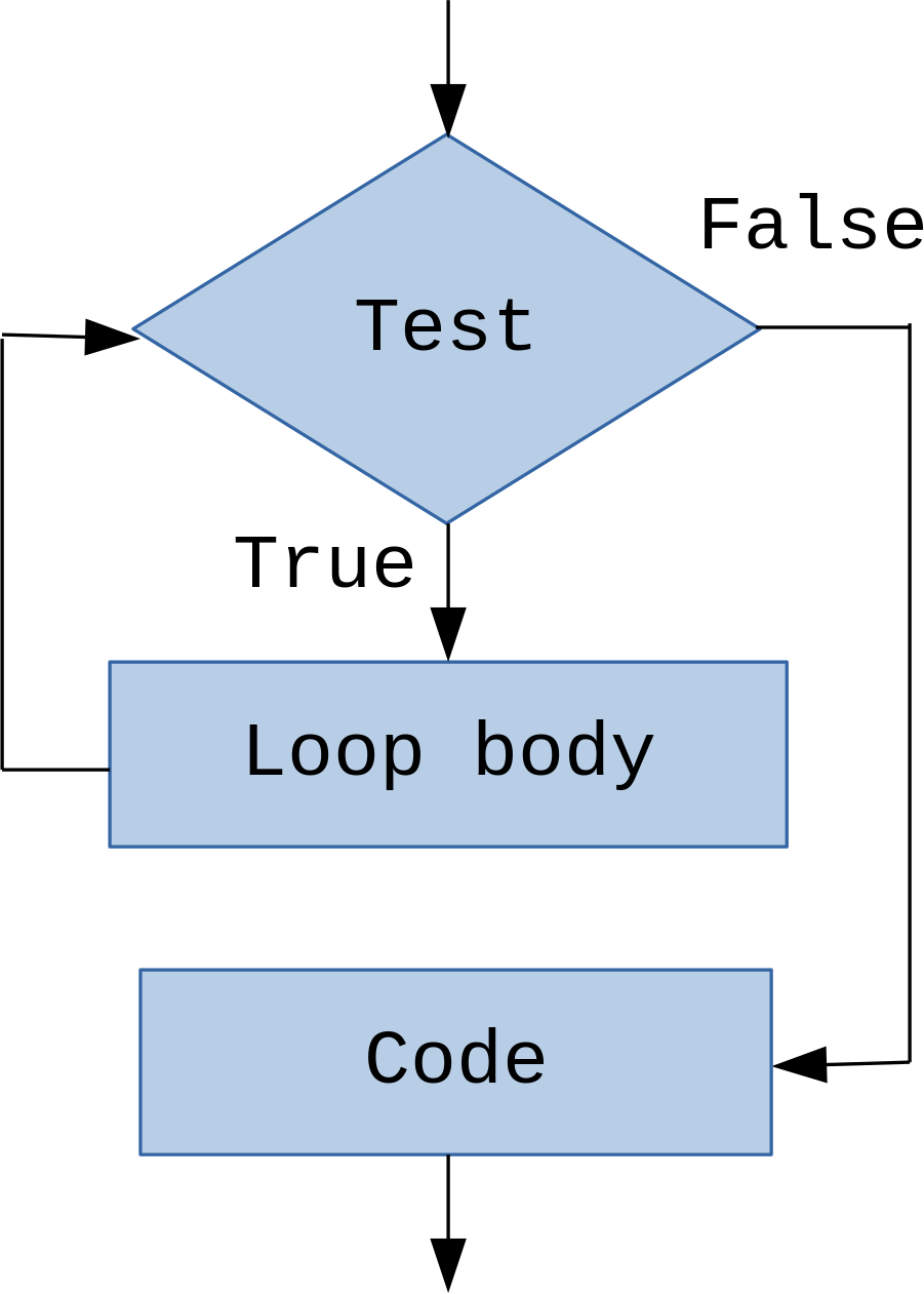
Algorithm flowchart (R)
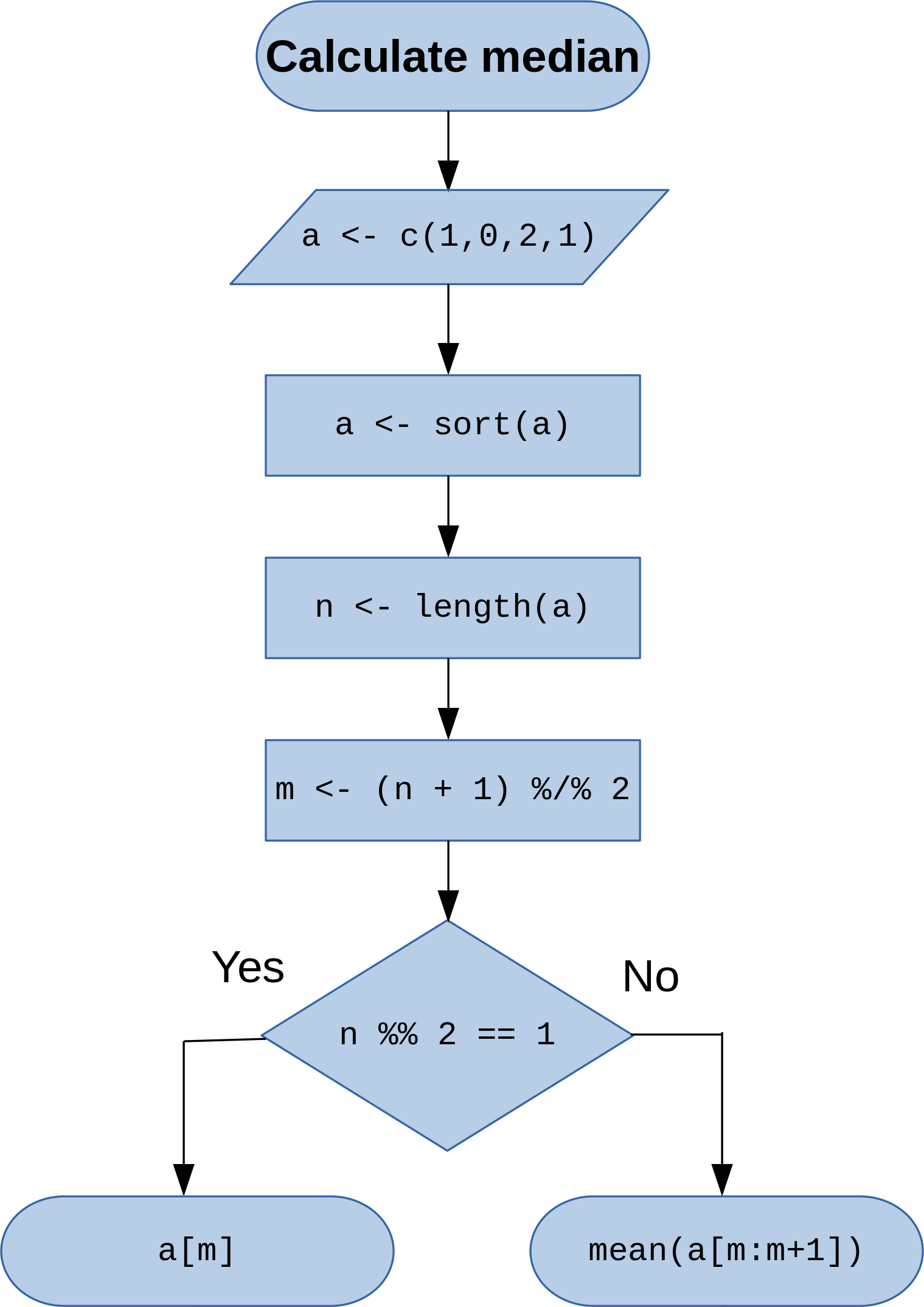
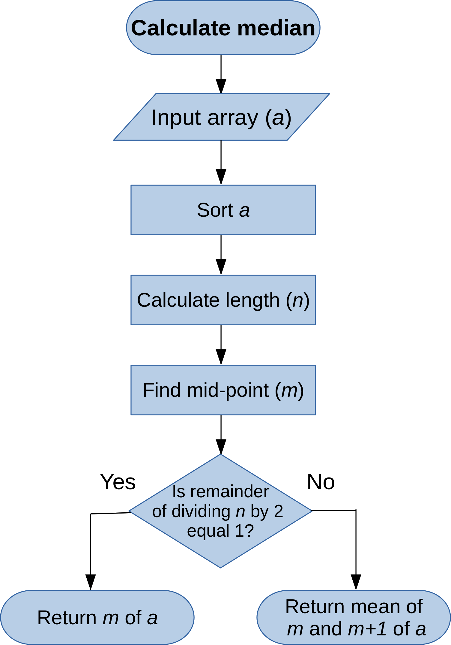
Calculate median
In [2]:
a <- c(1,0,2,1) # Input vector (1-dimensional array)
a <- sort(a) # Sort vector
a
[1] 0 1 1 2
In [3]:
n <- length(a) # Calculate length of vector 'a'
n
[1] 4
In [4]:
m <- (n + 1) %/% 2 # Calculate mid-point, %/% is operator for integer division
m
[1] 2
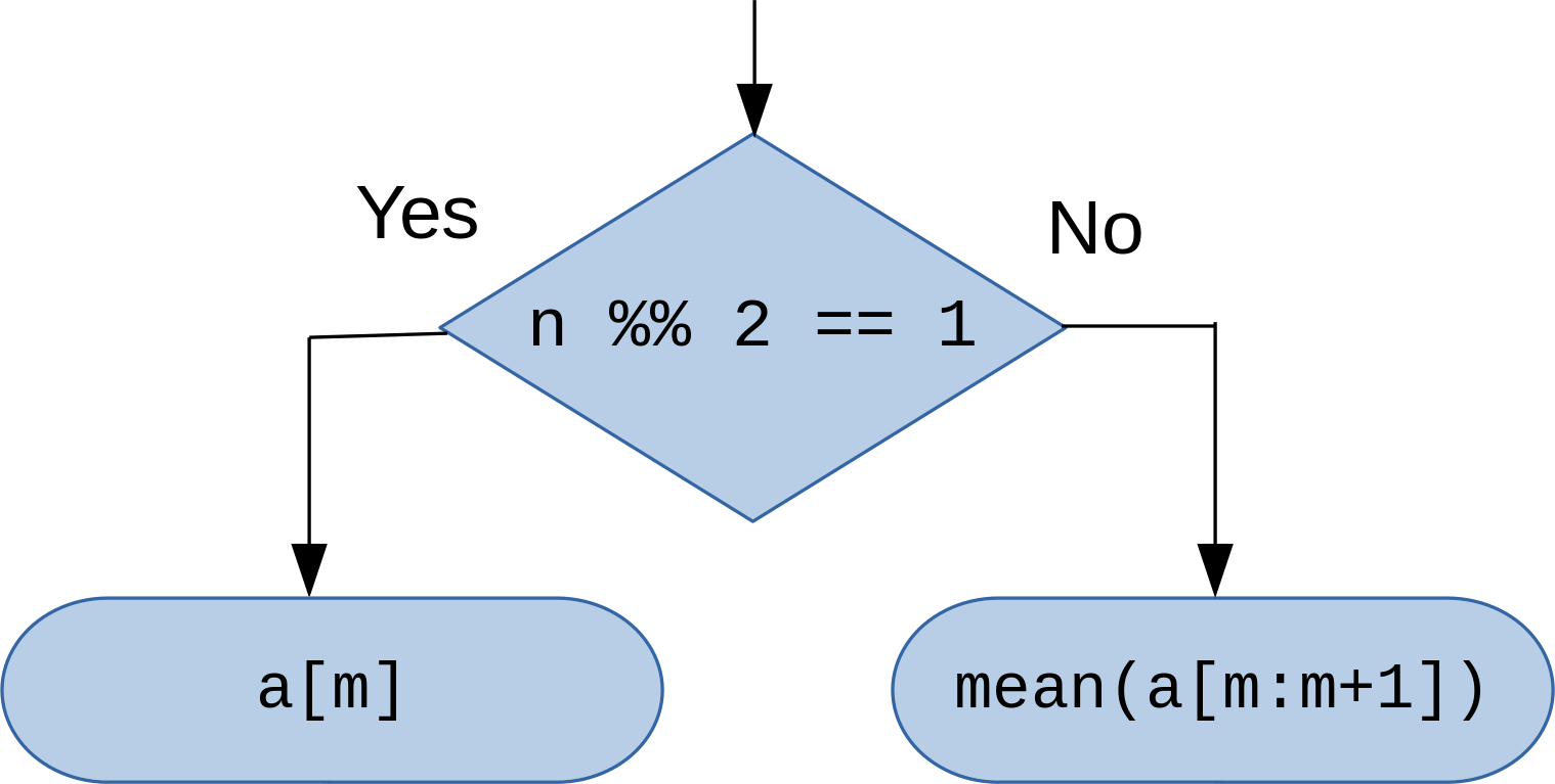
In [5]:
n %% 2 == 1 # Check whether the number of elements is odd, %% (modulo) gives remainder of division
[1] FALSE
In [6]:
mean(a[m:m+1])
[1] 1
Control flow in R
- Control flow is the order in which statements are executed or evaluated
- Main ways of control flow in R:
- Branching (conditional) statements (e.g.
if) - Iteration (loops) (e.g.
for) - Function calls (e.g.
length())
- Branching (conditional) statements (e.g.
Branching programs
Conditional statements
Conditional statements: if
if- defines condition under which some code is executed
if (<boolean_expression>) {
  <some_code>
}
In [7]:
a <- c(1, 0, 2, 1, 100)
a <- sort(a)
n <- length(a)
m <- (n + 1) %/% 2
if (n %% 2 == 1) {
  a[m]
}
[1] 1
Conditional statements: if - else
if - else- defines both condition under which some code is executed and alternative code to execute
if (<boolean_expression>) {
  <some_code>
} else {
  <some_other_code>
}
In [8]:
a <- c(1, 0, 2, 1)
a <- sort(a)
n <- length(a)
m <- (n + 1) %/% 2
if (n %% 2 == 1) {
  a[m]
} else {
  mean(a[m:m+1])
}
[1] 1
Conditional statements: if - else if - else
if - else if - ... - else- defines both condition under which some code is executed and several alternatives
if (<boolean_expression>) {
  <some_code>
} else if (<boolean_expression>) {
  <some_other_code>
} else if (<boolean_expression>) {
...
...
} else {
  <some_more_code>
}
Example of longer conditional statement
In [9]:
x <- 42
if (x > 0) {
  print("Positive")
} else if (x < 0) {
  print("Negative")
} else {
  print("Zero")
}
[1] "Positive"
Optimising conditional statements
- Parts of conditional statement are evaluated sequentially, so it makes sense to put the most likely condition as the first one
In [10]:
# Ask for user input and cast as double
num <- as.double(readline("Please, enter a number:"))
if (num %% 2 == 0) {
  print("Even")
} else if (num %% 2 == 1) {
  print("Odd")
} else {
  print("This is a real number")
}
Please, enter a number:43
[1] "Odd"
Nesting conditional statements
- Conditional statements can be nested within each other
- But consider code legibility 📜, modularity ⚙️ and speed 🏎️
In [11]:
num <- as.integer(readline("Please, enter a number:")) # Ask for user input and cast as integer
if (num > 0) {
  if (num %% 2 == 0) {
    print("Positive even")
  } else {
    print("Positive odd")
  }
} else if (num < 0) {
  if (num %% 2 == 0) {
    print("Negative even") # Notice that odd/even check appears twice
  } else {
    print("Negative odd") # Consider abstracting this as a function
  }
} else {
  print("Zero")
}
Please, enter a number:-43
[1] "Negative odd"
ifelse() function
- R also provides a vectorized version of
if - elseconstruct - It takes a vector as an input and returns another vector as an output
ifelse(<boolean_expression>, <if_true>, <if_false>)In [12]:
num <- 1:10
num
[1] 1 2 3 4 5 6 7 8 9 10
In [13]:
ifelse(num %% 2 == 0, "even", "odd")
[1] "odd" "even" "odd" "even" "odd" "even" "odd" "even" "odd" "even"
Iteration (looping)
Iteration: while
while- defines a condition under which some code (loop body) is executed repeatedly
while (<boolean_expression>) {
  <some_code>
}
In [14]:
# Calculate a factorial with decrementing function
# E.g. 5! = 1 * 2 * 3 * 4 * 5 = 120
x <- 5
factorial <- 1
while (x > 0) {
  factorial <- factorial * x
  x <- x - 1
}
factorial
[1] 120
Iteration: for
for- defines elements and sequence over which some code is executed iteratively
for (<element> in <sequence>) {
  <some_code>
}
In [15]:
x <- seq(5)
factorial <- 1
for (i in x) {
  factorial <- factorial * i
}
factorial
[1] 120
Iteration with conditional statements
In [16]:
# Find maximum value in a vector with exhaustive enumeration
v <- c(3, 27, 9, 42, 10, 2, 5)
max_val <- v[1]
for (i in v) {
  if (i > max_val) {
    max_val <- i
  }
}
max_val
[1] 42
Generating sequences for iteration
seq()function that we encountered in subsetting can be used in looping- As well as its cousins:
seq_len()andseq_along()
seq(<from>, <to>, <by>)
seq_len(<length>)
seq_along(<object>)
Generating sequences for iteration examples
In [17]:
# If by argument is omitted, it defaults to 1
s <- seq(25, 44)
s
[1] 25 26 27 28 29 30 31 32 33 34 35 36 37 38 39 40 41 42 43 44
In [18]:
# seq_len() is equivalent to seq(1, length(<object>))
seq_len(length(s))
[1] 1 2 3 4 5 6 7 8 9 10 11 12 13 14 15 16 17 18 19 20
In [19]:
seq_along(s)
[1] 1 2 3 4 5 6 7 8 9 10 11 12 13 14 15 16 17 18 19 20
In [20]:
# The sequence that you are supplying to seq_along() doesn't have to be numeric
seq_along(letters[1:20])
[1] 1 2 3 4 5 6 7 8 9 10 11 12 13 14 15 16 17 18 19 20
Generating sequences for iteration examples continued
In [21]:
# vector() function is useful for initiliazing empty vectors of known type and length
s2 <- vector(mode = "double", length = length(s))
for (i in seq_len(length(s))) {
    s2[i] <- s[i] * 2
}
In [22]:
s2
[1] 50 52 54 56 58 60 62 64 66 68 70 72 74 76 78 80 82 84 86 88
In [23]:
s3 <- vector(mode = "double", length = length(s))
for (i in seq_along(s)) {
    s3[i] <- s[i] * 3
}
In [24]:
s3
 [1]  75  78  81  84  87  90  93  96  99 102 105 108 111 114 117 120 123 126 129
[20] 132
Iteration: break and next
break- terminates the loop in which it is containednext- exits the iteration of a loop in which it is contained
In [25]:
for (i in seq(1,6)) {
  if (i %% 2 == 0) {
    break
  }
  print(i)
}
[1] 1
In [26]:
for (i in seq(1,6)) {
  if (i %% 2 == 0) {
    next
  }
  print(i)
}
[1] 1
[1] 3
[1] 5
Infinite loop
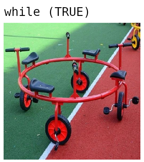
Infinite loops
- Loops that have no explicit limits for the number of iterations are called infinite
- They have to be terminated with a
breakstatement (or Ctrl/Cmd-C in interactive session) - Such loops can be unintentional (bug) or desired (e.g. waiting for user's input, some event)
In [27]:
i <- 1
while (TRUE) {
  i <- i + 1
  if (i > 10) {
    break
  }
}
In [28]:
i
[1] 11
Iteration: repeat
repeat- defines code which is executed iteratively until the loop is explicitly terminated- Is equivalent to
while (TRUE)
repeat {
  <some_code>
}
In [29]:
i <- 1
repeat {
  i <- i + 1
  if (i > 10) {
    break
  }
}
In [30]:
i
[1] 11

Decomposition and abstraction
- So far: built-in types, assignments, branching and looping constructs
- In principle, any problem can be solved just with those
- But a solution would be non-modual and hard-to-maintain
- Functions provide decomposition and abstraction
Functions in R
- Function call is the centerpiece of computation in R
- It involves function object and objects that are supplied as arguments
- Functions in R do not have side-effects (nonlocal modifications of input objects)
- In R we use function
function()to create a function object - Functions are also referred to as closures in some R documentation
<function_name> <- function(<arg_1>, <arg_2>, ..., <arg_n>) {
  <function_body>
}
In [31]:
foo <- function(arg) {
  # <function_body>
}
Function components
- Body (
body()) - code inside the function - List of arguments (
formals()) - controls how function is called - Environment/scope/namespace (
environment()) - location of function's definition and variables
Function components example
In [32]:
is_positive <- function(num) {
  if (num > 0) {
    return(TRUE)
  } else {
    return(FALSE)
  }
}
In [33]:
body(is_positive)
{
    if (num > 0) {
        return(TRUE)
    }
    else {
        return(FALSE)
    }
}
In [34]:
formals(is_positive)
$num
In [35]:
environment(is_positive)
<environment: R_GlobalEnv>
Function call
- Function is executed until:
- Either
return()function is encountered - There are no more expressions to evaluate
- Either
- Function call always returns a value:
- Argument of
return()function call - Value of last expression if no
return()(implicit return)
- Argument of
- Function can return only one object
- But you can combine multiple R objects in a list
Function call example
In [36]:
is_positive <- function(num) {
  if (num > 0) {
    res <- TRUE
  } else {
    res <- FALSE
  }
  return(res)
}
In [37]:
res_1 <- is_positive(5)
res_2 <- is_positive(-7)
In [38]:
print(res_1)
print(res_2)
[1] TRUE
[1] FALSE
Implicit return example
In [39]:
is_positive <- function(num) {
  if (num > 0) {
    res <- TRUE
  } else {
    res <- FALSE
  }
  res
}
In [40]:
res_1 <- is_positive(5)
res_2 <- is_positive(-7)
In [41]:
print(res_1)
print(res_2)
[1] TRUE
[1] FALSE
Implicit return example continued
In [42]:
# While this function provides the same functionality as the two versions above
# This is an example of a bad programming style, return value is very unintuitive
is_positive <- function(num) {
  if (num > 0) {
    res <- TRUE
  } else {
    res <- FALSE
  }
}
In [43]:
res_1 <- is_positive(5)
res_2 <- is_positive(-7)
In [44]:
print(res_1)
print(res_2)
[1] TRUE
[1] FALSE
Function arguments
- Arguments provide a way of giving input to a function
- Arguments in function definition are formal arguments
- Arguments in function invocations are actual arguments
- When a function is invoked (called) arguments are matched and bound to local variable names
- R matches arguments in 3 ways:
- by exact name
- by partial name
- by position
- It is a good idea to only use unnamed (positional) for the main (first one or two) arguments
Function arguments example
In [45]:
format_date <- function(day, month, year, reverse = TRUE) {
  if (isTRUE(reverse)) {
    formatted <- paste(
      as.character(year), as.character(month), as.character(day), sep = "-"
    )
  } else {
    formatted <- paste(
      as.character(day), as.character(month), as.character(year), sep = "-"
    )
  }
  return(formatted)
}
In [46]:
format_date(4, 10, 2021)
[1] "2021-10-4"
In [47]:
format_date(y = 2021, m = 10, d = 4) # Technically correct, but rather unintuitive
[1] "2021-10-4"
In [48]:
format_date(y = 2021, m = 10, d = 4, FALSE) # Technically correct, but rather unintuitive
[1] "4-10-2021"
In [49]:
format_date(day = 4, month = 10, year = 2021, FALSE)
[1] "4-10-2021"
Nested functions
In [50]:
which_integer <- function(num) {
  even_or_odd <- function(num) {
    if (num %% 2 == 0) {
      return("even")
    } else {
      return("odd")
    }
  }
  eo <- even_or_odd(num)
  if (num > 0) {
    return(paste0("positive ", eo))
  } else if (num < 0) {
    return(paste0("negative ", eo))
  } else {
    return("zero")
  }
}
In [51]:
which_integer(-43)
[1] "negative odd"
In [52]:
even_or_odd(-43)
Error in even_or_odd(-43): could not find function "even_or_odd"
Traceback:
R environment basics
- Variables (aka names) exist in an environment (aka namespace/scope in Python)
- The same R object can have different names
- Binding of objects to names (assignment) happens within a specific environment
- Most environments get created by function calls
- Approximate hierarchy of environments:
- Execution environment of a function
- Global environment of a script
- Package environment of any loaded packages
- Base environment of base R objects
R environment example
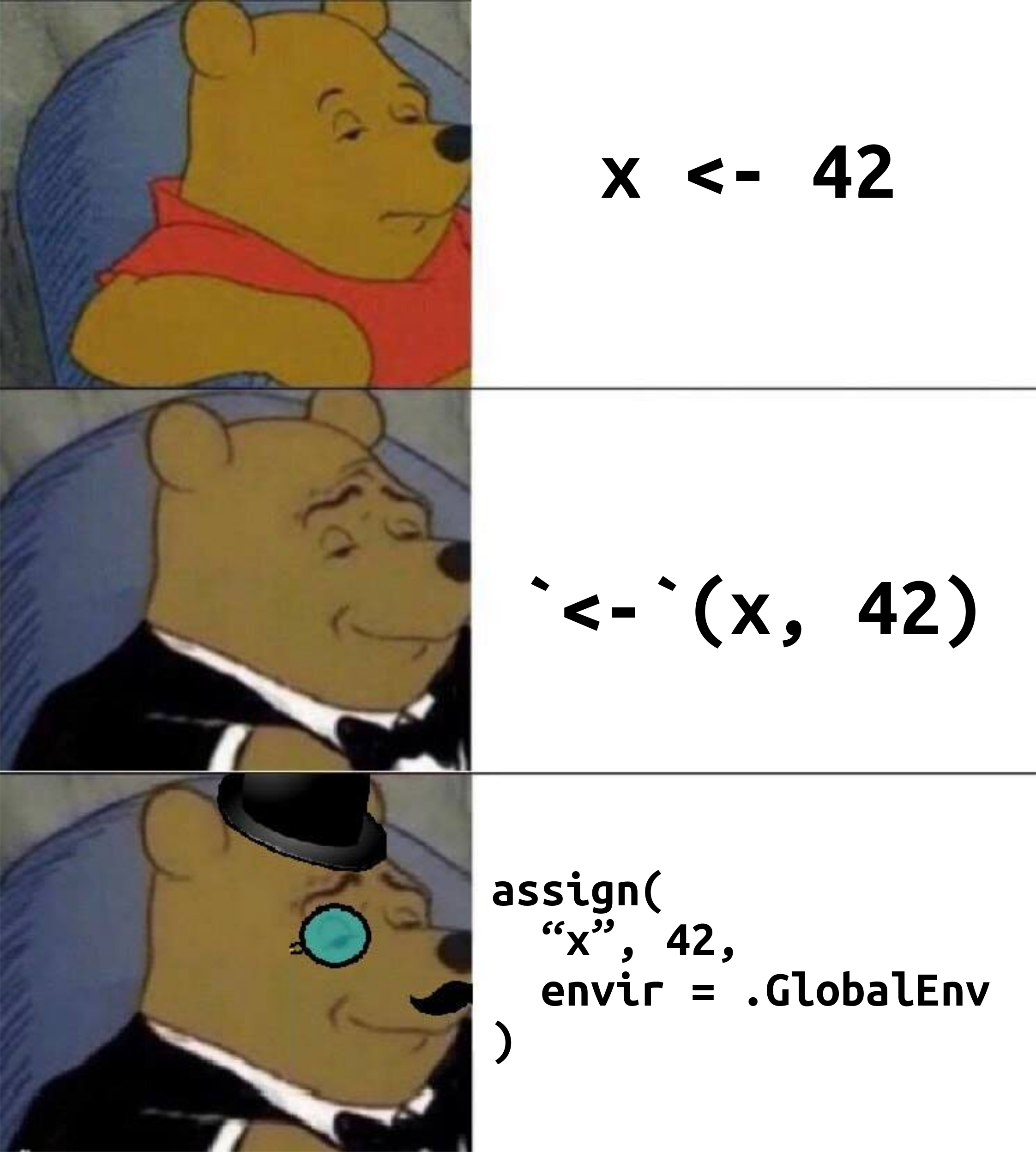
In [53]:
x <- 42
# is equivalent to:
# Binding R object '42', double vector of length 1, to name 'x' in the global environment
assign("x", 42, envir = .GlobalEnv)
x
[1] 42
In [54]:
x <- 5
foo <- function() {
  x <- 12
  return(x)
}
y <- foo()
print(y)
print(x)
[1] 12
[1] 5
Examples of operators as function calls
In [55]:
`+`(3, 2) # Equivalent to: 3 + 2
[1] 5
In [56]:
`<-`(x, c(10, 12, 14)) # x <- c(10, 12, 14)
x
[1] 10 12 14
In [57]:
`[`(x, 3) # x[3]
[1] 14
In [58]:
`>`(x, 10) # x > 10
[1] FALSE TRUE TRUE
Anonymous functions
- While R has no special syntax for creating anonymous (aka lambda in Python) function
- Note that the result of
function()does not have to be assigned to a variable - Thus function
function()can be easily incorporate into other function calls
In [59]:
add_five <- function() {
  return(function(x) x + 5)
}
af <- add_five()
In [60]:
af # 'af' is just a function, which is yet to be invoked (called)
function(x) x + 5
<environment: 0x55baf8cccac0>
In [61]:
af(10) # Here we call a function and supply 10 as an argument
[1] 15
In [62]:
# Due to vectorized functions in R this example is an obvious overkill (seq(10) ^ 2 would do just fine)
# but it shows a general approach when we might need to apply a non-vectorized functions
sapply(seq(10), function(x) x ^ 2)
[1] 1 4 9 16 25 36 49 64 81 100
Functionals
- Functionals are functions that take other functions as one of their inputs
- Due to R's functional nature, functionals are frequently used for many tasks
apply()family of base R functionals is the most ubiquitous example- Their most common use case is an alternative of for loops
- Loops in R have a reputation of being slow (not always warranted)
- Functionals also allow to keep code more concise
Functional example
In [63]:
# Applies a supplied function to a random draw
# from the normal distribution with mean 0 and sd 1
functional <- function(f) { f(rnorm(10)) }
In [64]:
functional(mean)
[1] 0.3186378
In [65]:
functional(median)
[1] -0.2481884
In [66]:
functional(sum)
[1] 1.492055
Summary of common apply() functions
| Function | Description | Input Object | Output Object | Simplified |
|---|---|---|---|---|
apply() |
Apply a given function to margins (rows/columns) of input object | matrix/array/data.frame | vector/matrix/array/list | Yes |
lapply() |
Apply a given function to each element of input object | vector/list | list | No |
sapply() |
Same as lapply(), but output is simplified |
vector/list | vector/matrix | Yes |
vapply() |
Same as sapply(), but data type of output is specified |
vector/list | vector | No |
mapply() |
Multivariate version of sapply(), takes multiple objects as input |
vectors/lists | vector/matrix | Yes |
lapply() function
- Takes a function and a vector or list as input
- Applies the input function to each element in the list
- Returns list as an onput
lapply(<input_object>, <function_name>, <arg_1>, ..., <arg_n>)lapply() examples
In [67]:
l <- list(a = 1:2, b = 3:4, c = 5:6, d = 7:8, e = 9:10)
In [68]:
# Apply sum() to each element of list 'l'
lapply(l, sum)
$a
[1] 3

$b
[1] 7

$c
[1] 11

$d
[1] 15

$e
[1] 19
In [69]:
# We can exploit the fact that basic operators are function calls
# Here, each subsetting operator `[` with argument 2 is applied to each element
# Which gives us second element within each element of the list
lapply(l, `[`, 2)
$a
[1] 2

$b
[1] 4

$c
[1] 6

$d
[1] 8

$e
[1] 10
apply() function
- Works with higher-dimensional (> 1d) input objects (matrices, arrays, data frames)
- Is a common tool for calculating summaries of rows/columns
<margin>argument indicates whether function is applied across rows (1) or columns (2)
apply(<input_object>, <margin>, <function_name>, <arg_1>, ..., <arg_n>)apply() examples
In [70]:
m <- matrix(1:12, nrow = 3, ncol = 4)
m
     [,1] [,2] [,3] [,4]
[1,] 1    4    7    10
[2,] 2    5    8    11
[3,] 3    6    9    12
In [71]:
# Sum up rows (can also be achieved with rowSums() function)
apply(m, 1, sum)
[1] 22 26 30
In [72]:
# Calculate averages across columns (also available in colMeans())
apply(m, 2, mean)
[1] 2 5 8 11
In [73]:
# Find maximum value in each column
apply(m, 2, max)
[1] 3 6 9 12
mapply() function
- Takes a function and multiple vectors or lists as input
- Applies the function to each corresponding element of input sequences
- Simplifies output into vector (if possible)
mapply(<function_name>, <input_object_1>, ..., <input_object_n>, <arg_1>, ..., <arg_n>)mapply() examples
In [74]:
means <- -2:2
sds <- 1:5
In [75]:
# Generate one draw from a normal distribution where
# each mean is an element of vector 'means'
# and each standard deivation is an element of vector 'sds'
#
# rnorm(n, mean, sd) takes 3 arguments: n, mean, sd

mapply(rnorm, 1, means, sds)
[1] -0.7043966 -2.9181125 0.7705752 0.8115289 4.9755344
In [76]:
# While simplification of output
# (attempt to collapse it in fewer dimensions)
# makes hard to predict the object returned
# by apply() functions that have simplified = TRUE by default

mapply(rnorm, 5, means, sds)
     [,1]      [,2]       [,3]        [,4]       [,5]
[1,] -3.058834 -1.0853410 -0.08222913 -0.6397508  1.8098831
[2,] -2.759082 -3.6308276 -1.53727082  1.4870609 -0.4620664
[3,] -1.633935 -0.1775828 -3.99636499  2.7069711  4.1554896
[4,] -1.241012 -1.8139769 -0.35165313  5.2904383 11.1715264
[5,] -1.227846 -1.5496606  2.82421174  5.9838118  4.9411164
Packages
- Program can access functionality of a package using
library()function - Every package has its own namespace (which can accessed with
::)
library(<package_name>)
<package_name>::<object_name>
Package loading example
In [77]:
# Package 'Matrix' is part of the standard R library and doesn't have to be installed separately
library("Matrix")
In [78]:
# While it is possible to just use function sparseVector() after loading the library,
# it is good practice to state explicitly which package the object is coming from.
sv <- Matrix::sparseVector(x = c(1, 2, 3), i = c(3, 6, 9), length = 10)
In [79]:
sv
sparse vector (nnz/length = 3/10) of class "dsparseVector"
 [1] . . 1 . . 2 . . 3 .
Next
- Data wrangling