Overview
- Software bugs
- Debugging
- Handling conditions
- Testing
- Defensive programming

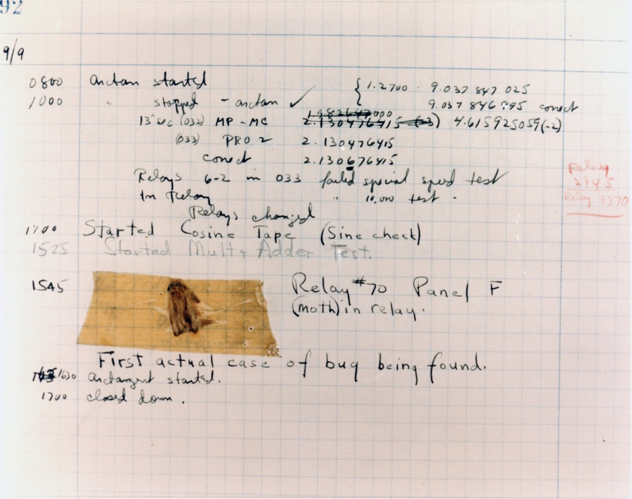
Computer bugs before
 |
 |
Grace Murray Hopper popularised the term bug after in 1947 her team traced an error in the Mark II to a moth trapped in a relay.
Computer bugs today
In [2]:
even_or_odd <- function(num) {
  if (num %% 2 == 0) {
    return("even")
  } else {
    return("odd")
  }
}
In [3]:
even_or_odd(42.7)
[1] "odd"
In [4]:
even_or_odd('42')
Error in num%%2: non-numeric argument to binary operator
Traceback:

1. even_or_odd("42")
Explicit expectations
In [5]:
even_or_odd <- function(num) {
  num <- as.integer(num) # We expect input to be integer or convertible into one
  if (num %% 2 == 0) {
    return("even")
  } else {
    return("odd")
  }
}
In [6]:
even_or_odd(42.7)
[1] "even"
In [7]:
even_or_odd('42')
[1] "even"
Types of bugs
- Overt vs covert
- Overt bugs have obvious manifestation (e.g. premature program termination, crash)
- Covert bugs manifest themselves in wrong (unexpected) results
- Persistent vs intermittent
- Persistent bugs occur for every run of the program with the same input
- Intermittent bugs occur occasionally even given the same input and other conditions

Debugging
Fixing a buggy program is a process of confirming, one by one, that the many things you believe to be true about the code actually are true. When you find that one of your assumptions is not true, you have found a clue to the location (if not the exact nature) of a bug.
Norman Matloff
- Process of finding, isolating and fixing an existing problem in computer program
Debugging process
- Realise that you have a bug
- Could be non-trivial for covert and intermittent bugs
- Make it reproducible
- Extremely important step that makes debugging easier
- Isolate the smallest snippet of code that repeats the bug
- Test with different inputs/objects
- Will also be helpful if you are seeking outside help
- Provides a case that can be used in automated testing
- Figure out where it is
- Formulate hypotheses, design experiments
- Test hypotheses on a reproducible example
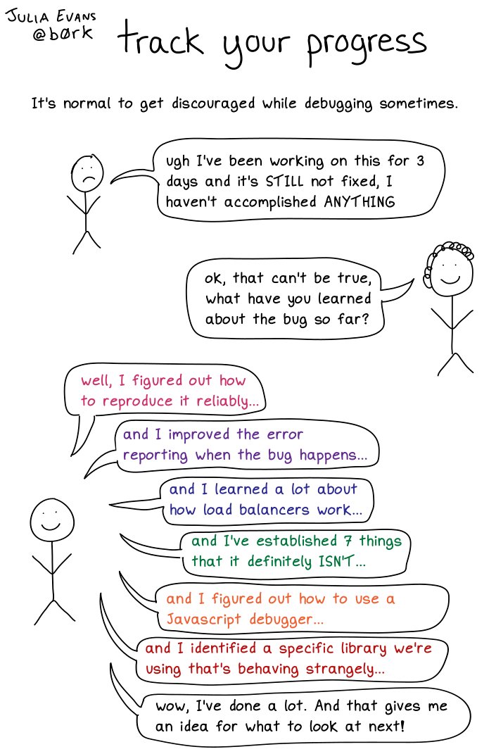
- Keep track of the solutions that you have attempted
- If it worked:
- Fix the bug and test the use-case
- Otherwise:
- Sleep on it
Debugging with print()
print()statement can be used to check the internal state of a program during evaluation- Can be placed in critical parts of code (before or after loops/function calls/objects loading)
- Can be combined with function
ls()(andget()/mget()) to reveal all local objects - For harder cases switch to R debugging functions(
debug()/debugonce())
Bug example
In [8]:
calculate_median <- function(a) {
  a <- sort(a)
  n <- length(a)
  m <- (n + 1) %/% 2
  if (n %% 2 == 1) {
    med <- a[m]
  } else {
    med <- a[m-1:m]
  }
  return(med)
}
In [9]:
v1 <- c(1, 2, 3)
v2 <- c(0, 1, 1, 2)
In [10]:
calculate_median(v1)
[1] 2
In [11]:
calculate_median(v2)
[1] 0
Debugging with print() example
In [12]:
calculate_median <- function(a) {
  a <- sort(a)
  n <- length(a)
  m <- (n + 1) %/% 2
  print(m)
  if (n %% 2 == 1) {
    med <- a[m]
  } else {
    med <- a[m-1:m]
  }
  return(med)
}
In [13]:
v1 <- c(1, 2, 3)
v2 <- c(0, 1, 1, 2)
In [14]:
calculate_median(v1)
[1] 2
[1] 2
In [15]:
calculate_median(v2)
[1] 2
[1] 0
Debugging with print() and ls() example
In [16]:
calculate_median <- function(a) {
  a <- sort(a)
  n <- length(a)
  m <- (n + 1) %/% 2
  # Analogous to Python's print(vars())
  # Print all objects in function environment
  print(mget(ls()))
  if (n %% 2 == 1) {
    med <- a[m]
  } else {
    med <- a[m-1:m]
  }
  return(med)
}
In [17]:
calculate_median(v1)
$a
[1] 1 2 3

$m
[1] 2

$n
[1] 3
[1] 2
In [18]:
calculate_median(v2)
$a
[1] 0 1 1 2

$m
[1] 2

$n
[1] 4
[1] 0
Debugging with print() example continued
In [19]:
calculate_median <- function(a) {
  a <- sort(a)
  n <- length(a)
  m <- (n + 1) %/% 2
  if (n %% 2 == 1) {
    med <- a[m]
  } else {
    print(m-1:m)
    med <- a[m-1:m]
  }
  return(med)
}
In [20]:
calculate_median(v1)
[1] 2
In [21]:
calculate_median(v2)
[1] 1 0
[1] 0
Fixing a bug and testing
In [22]:
calculate_median <- function(a) {
  a <- sort(a)
  n <- length(a)
  m <- (n + 1) %/% 2
  if (n %% 2 == 1) {
    med <- a[m]
  } else {
    med <- a[m:m+1]
  }
  return(med)
}
In [23]:
calculate_median(v1)
[1] 2
In [24]:
calculate_median(v2)
[1] 1
R Debugging Facilities
- The core of R debugging process is stepping through the code as it gets executed
- This permits the inspection of the environment where a problem occurs
- Three functions provide the the main entries into the debugging mode:
browser()- pauses the execution at a dedicated line in code (breakpoint)debug()/undebug()- (un)sets a flag to run function in a debug mode (setting through)debugonce()- triggers single stepping through a function
Breakpoints
In [25]:
calculate_median <- function(a) {
  a <- sort(a)
  n <- length(a)
  m <- (n + 1) %/% 2
  if (n %% 2 == 1) {
    med <- a[m]
  } else {
    browser()
    med <- a[m-1:m]
  }
  return(med)
}
In [26]:
## Example for running in RStudio
calculate_median(v2)
Called from: calculate_median(v2)
debug at <text>#9: med <- a[m - 1:m]
debug at <text>#11: return(med)
[1] 0
Debugger commands
| Command | Description |
|---|---|
n(ext) |
Execute next line of the current function |
s(tep) |
Execute next line, stepping inside the function (if present) |
c(ontinue) |
Continue execution, only stop when breakpoint in encountered |
f(inish) |
Finish execution of the current loop or function |
Q(uit) |
Quit from the debugger, executed program is aborted |
Conditions
- Conditions are events that signal special situations during execution
- Some conditions can modify the control flow of a program (e.g. error)
- They can be caught and handled by your code
- You can also incorporate condition triggers into your code
Extra: Hadley Wickham - Conditions
Conditions examples
In [27]:
42 + "ab" # Throws an error
Error in 42 + "ab": non-numeric argument to binary operator
Traceback:
In [28]:
as.numeric(c("42", "55.3", "ab", "7")) # Triggers a warning
Warning message in eval(expr, envir, enclos):
“NAs introduced by coercion”
[1] 42.0 55.3 NA 7.0
In [29]:
library("dplyr") # Shows a message
Attaching package: ‘dplyr’


The following objects are masked from ‘package:stats’:

    filter, lag


The following objects are masked from ‘package:base’:

    intersect, setdiff, setequal, union
Conditions examples continued
In [30]:
stop("This is what an error looks like")
Error in eval(expr, envir, enclos): This is what an error looks like
Traceback:

1. stop("This is what an error looks like")
In [31]:
warning("This is what a warning looks like")
Warning message in eval(expr, envir, enclos):
“This is what a warning looks like”
In [32]:
message("This is what a message looks like")
This is what a message looks like
Errors
- In R errors are signalled (or thrown) with
stop() - By default, the error message includes the call.
- Program execution stops once an error is raised
In [33]:
if (c(TRUE, TRUE, FALSE)) {
  print("This used to word pre R-4.2.0")
}
Error in if (c(TRUE, TRUE, FALSE)) {: the condition has length > 1
Traceback:
Warnings
- Weaker versions of errors:
- Something went wrong, but the program has been ableto recover and continue.
- Single call in result in multiple warnings (as opposed to a single error).
- Take note of the warnings resulting from base R operations.
- Some of them might eventually become errors.
In [34]:
# Will become an error in future versions of R
c(TRUE, FALSE) && c(TRUE, TRUE)
Warning message in c(TRUE, FALSE) && c(TRUE, TRUE):
“'length(x) = 2 > 1' in coercion to 'logical(1)'”
Warning message in c(TRUE, FALSE) && c(TRUE, TRUE):
“'length(x) = 2 > 1' in coercion to 'logical(1)'”
[1] TRUE
Messages
- Messages serve mostly informational purposes.
- They tell the user:
- that something was done
- the details of how something was done.
- Sometimes these actions are not anticipated.
- Useful for functions with side-effects (accessing server, writing to disk, etc.)
In [35]:
anscombes_quartet <- readr::read_csv("../data/anscombes_quartet.csv")
Rows: 44 Columns: 3
── Column specification ───────────────────────────────────────────────────────────────────────────────────────────────────────────────────────────────────────────────────────────────────────────────────────────
Delimiter: ","
chr (1): dataset
dbl (2): x, y

ℹ Use `spec()` to retrieve the full column specification for this data.
ℹ Specify the column types or set `show_col_types = FALSE` to quiet this message.
Handling conditions
- Every condition has default behaviour:
- Errors terminate program execution
- Warnings are captured and displayed in aggregate
- Message are shown immediately
- But with condition handlers we can override the default behaviour.
Ignoring conditions
- The simplest way of handling conditions is ignoring them.
- Heavy-handed approach, given the type of condition does not make further distinctions.
- Bear in mind the risks of ignoring the information (especially, errors!)
- Functions for handling conditions depend on the type of condition:
try()for errorssuppressWarnings()for warningssuppressMessages()for messages
In [36]:
suppressMessages(anscombes_quartet <- readr::read_csv("../data/anscombes_quartet.csv"))
In [37]:
# But some functions would provide arguments to silence messages
# This should be preferred to heavy-handed suppressMessages()
anscombes_quartet <- readr::read_csv("../data/anscombes_quartet.csv", show_col_types = FALSE)
In [38]:
# suppressPackageStartupMessages() - a variant for package startup messages
# But suppressMessages() would also work.
suppressPackageStartupMessages(library("dplyr"))
Ignoring errors
In [39]:
f1 <- function(x) {
  log(x)
  10
}
In [40]:
f1("x")
Error in log(x): non-numeric argument to mathematical function
Traceback:

1. f1("x")
In [41]:
f2 <- function(x) {
  try(log(x))
  10
}
In [42]:
f2("y")
Error in log(x) : non-numeric argument to mathematical function
[1] 10
Condition handlers
- More advanced approach to dealing with conditions is providing handlers.
- They allow to override or supplement the default behaviour.
- In particular, two function can:
tryCatch()define exiting handlerswithCallingHandlers()define calling handlers
tryCatch(
  error = function(cnd) {
    # code to run when error is thrown
  },
  code_to_run_while_handlers_are_active
)
withCallingHandlers(
warning = function(cnd) {
# code to run when warning is signalled
},
message = function(cnd) {
# code to run when message is signalled
},
code_to_run_while_handlers_are_active
)Exiting handlers
- The handlers set up by
tryCatch()are called exiting handlers. - After the condition is signalled, control flow passes to the handler.
- It never returns to the original code, effectively meaning that the code exits.
In [43]:
f3 <- function(x) {
  tryCatch(
    error = function(e) NA,
    log(x)
  )
}
In [44]:
f3("x")
[1] NA
Calling handlers
- With calling handlers code execution continues normally once the handler returns.
- A more natural pairing with the non-error conditions.
In [45]:
# Infinite loop, analogous to while (TRUE)
repeat {
  num <- readline("Please, enter a number:")
  if (num != "") {
    withCallingHandlers(
      warning = function(cnd) {
        print("This is not a number. Please, try again.")
      },
      num <- as.numeric(num)
    )
  } else {
    print("No input provided. Please, try again.")
  }
  if (!is.na(num)) {
    print(paste0("Your input '", as.character(num), "' is recorded"))
    break
  }
}
Please, enter a number:f
[1] "This is not a number. Please, try again."
Warning message in withCallingHandlers(warning = function(cnd) {:
“NAs introduced by coercion”
Please, enter a number:43
[1] "Your input '43' is recorded"
Testing
- Process of running a program on pre-determined cases to ascertain that its functionality is consistent with expectations
- Test cases consist of different assertions (of equality, boolean values, etc.)
- Fully-featured unit testing framework in R is provided in
testthatlibrary
Extra: Hadley Wickham - Testing
Testing examples
In [46]:
library("testthat")
Attaching package: ‘testthat’


The following object is masked from ‘package:dplyr’:

    matches
In [47]:
calculate_median <- function(a) {
  a <- sort(a)
  n <- length(a)
  m <- (n + 1) %/% 2
  if (n %% 2 == 1) {
    med <- a[m]
  } else {
    med <- a[m:m+1]
  }
  return(med)
}
In [48]:
testthat::test_that("The length of result is 1", {
  testthat::expect_equal(length(calculate_median(c(0, 1, 1, 2))), 1L)
  testthat::expect_equal(length(calculate_median(c(1, 2, 3))), 1L)
  testthat::expect_equal(length(calculate_median(c("a", "bc", "xyz"))), 1L)
})
Test passed 🥳
Testing examples continued
In [49]:
testthat::test_that("The result is numeric", {
  testthat::expect_true(is.numeric(calculate_median(c(0, 1, 1, 2))))
  testthat::expect_true(is.numeric(calculate_median(c(1, 2, 3))))
  testthat::expect_true(is.numeric(calculate_median(c("a", "bc", "xyz"))))
})
── Failure (<text>:4:3): The result is numeric ─────────────────────────────────
is.numeric(calculate_median(c("a", "bc", "xyz"))) is not TRUE

`actual`:   FALSE
`expected`: TRUE
Error:
! Test failed
Traceback:

1. testthat::test_that("The result is numeric", {
 .     testthat::expect_true(is.numeric(calculate_median(c(0, 1,
 .         1, 2))))
 .     testthat::expect_true(is.numeric(calculate_median(c(1, 2,
 .         3))))
 .     testthat::expect_true(is.numeric(calculate_median(c("a",
 .         "bc", "xyz"))))
 . })
2. (function (envir)
 . {
 .     handlers <- get_handlers(envir)
 .     errors <- list()
 .     for (handler in handlers) {
 .         tryCatch(eval(handler$expr, handler$envir), error = function(e) {
 .             errors[[length(errors) + 1]] <<- e
 .         })
 .     }
 .     attr(envir, "withr_handlers") <- NULL
 .     for (error in errors) {
 .         stop(error)
 .     }
 . })(<environment>)
Defensive programming
- Design your program to facilitate earlier failures, testing and debugging.
- Make code fail fast and in well-defined manner.
- Split up different componenets into functions or modules.
- Be strict about accepted inputs, use assertions or conditional statements to check them.
- Document assumptions and acceptable inputs using docstrings.
- Document non-trivial, potentially problematic and complex parts of code.