Week 3: Distributions & Sampling

POP88162 Introduction to Quantitative Research Methods

Working with Vectors

Let’s start by generating a random draw from a standard normal distribution

draws <- rnorm(100)

Check the top and bottom of this vector. Functions head() and tail() are applicable to different data structures in R. And printing out all 100 elements of this vector might be too verbose.

head(draws)

[1]  1.02144342 -0.31243248  1.73995487  1.02001652 -1.26753977  0.05604435

tail(draws)

[1] -0.1605959  0.2378662 -0.0554478 -1.3608837  1.0385050  0.7243626

Let’s practice more vector subsetting. How many of the numbers in this random draw are larger than 1?

draws > 1

  [1]  TRUE FALSE  TRUE  TRUE FALSE FALSE FALSE FALSE FALSE FALSE FALSE FALSE
 [13] FALSE FALSE FALSE  TRUE FALSE FALSE FALSE FALSE FALSE  TRUE FALSE FALSE
 [25] FALSE FALSE FALSE FALSE FALSE FALSE FALSE FALSE FALSE FALSE  TRUE FALSE
 [37] FALSE  TRUE FALSE FALSE FALSE FALSE FALSE FALSE FALSE  TRUE FALSE FALSE
 [49] FALSE FALSE FALSE FALSE FALSE FALSE FALSE FALSE FALSE FALSE FALSE FALSE
 [61] FALSE FALSE FALSE FALSE FALSE FALSE  TRUE  TRUE  TRUE FALSE FALSE FALSE
 [73] FALSE  TRUE FALSE FALSE FALSE FALSE FALSE FALSE FALSE FALSE FALSE FALSE
 [85] FALSE FALSE FALSE FALSE FALSE FALSE FALSE  TRUE FALSE FALSE FALSE FALSE
 [97] FALSE FALSE  TRUE FALSE

draws[draws > 1]

 [1] 1.021443 1.739955 1.020017 1.350512 1.915853 1.852528 1.096909 1.507518
 [9] 1.768061 3.096580 1.087257 1.494832 1.047338 1.038505

length(draws[draws > 1])

[1] 14

What proportion of random numbers is smaller than -3?

Working with Distributions

Let’s plot the density of a standard normal distribution. First, let’s, replicate the plot from the workshop by using dnorm() function.

x <- seq(-5, 5, 0.1)
plot(x, dnorm(x), type = "l")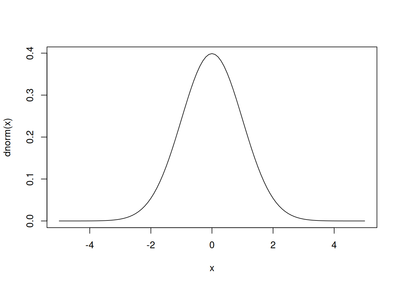

We can also get this plot by using random draws from above and built-in density() function in R. You can see that this plot is not nearly as pretty as the one above. This is due to a limited size of a random draw (only 100 observations). Try increasing the size of a random draw to check whether you can make this plot look closer to an ‘ideal’ normal distribution.

dens <- density(draws)
plot(dens)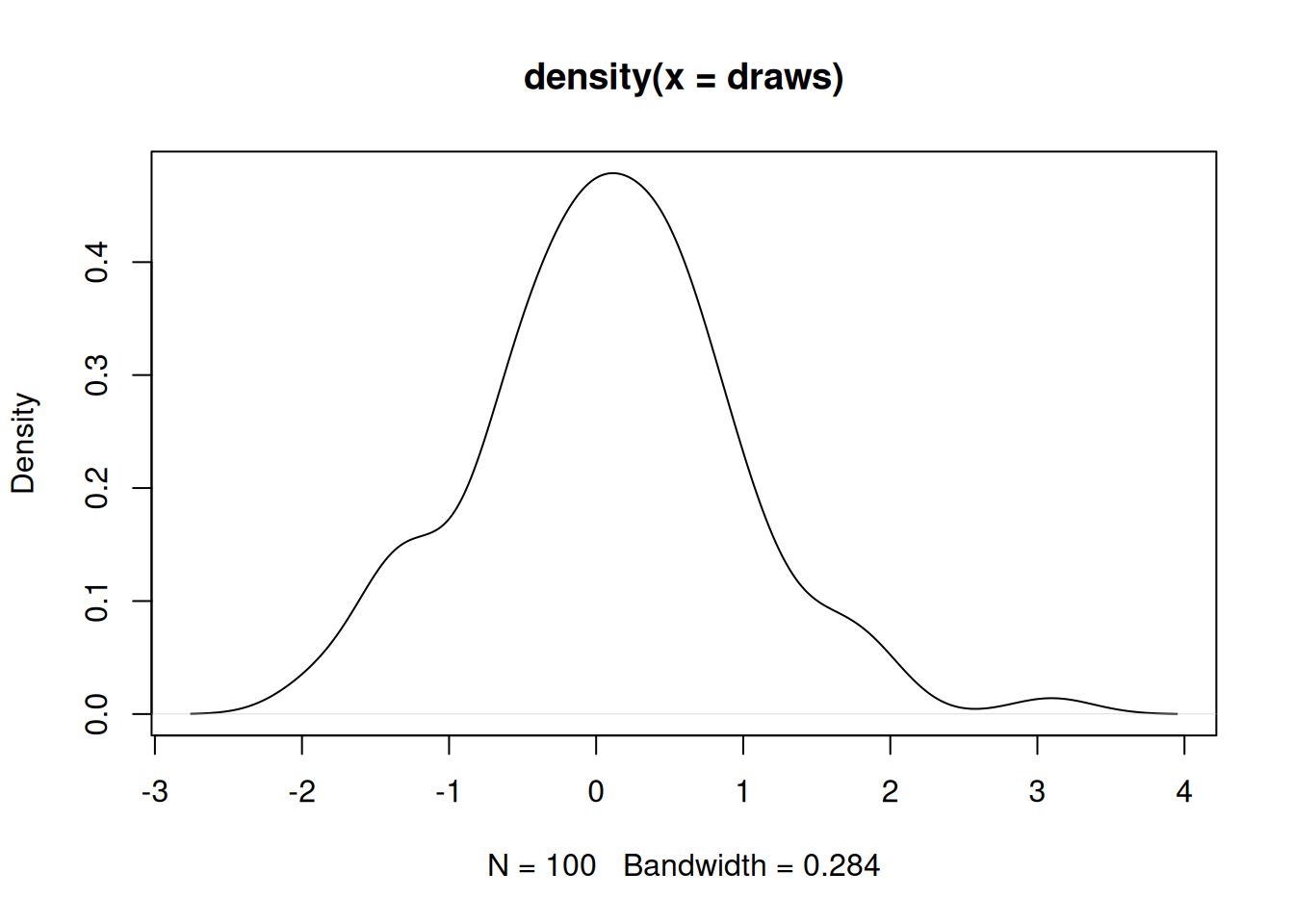

Plot a normal distribution with mean 10 and standard deviation 3.

Calculating probability

Following the example from the workshop, calculate the probability of observing a value larger than 2 for a variable that has a standard normal distribution.

Sampling

Function sample() often comes in handy when we need to draw a random sample from a dataset or an individual variable.

# Here, we are drawing a random sample of 5 from the vector `draws` created above
sample(draws, size = 5)

[1] -0.49966664  0.05604435  0.22929608 -0.37915400  0.23786624

Here is how we can draw a random sample from a data frame.

# Function with() tells R to obtain the variable names from `dens` object
# Otherwise, we would have needed to write its name twice and use $ subsetting
# as it is a list.
dd <- with(dens, data.frame(x, y))

# We are instructing R to draw a random sample of 10
# from the vector of row indices 1:nrow(dd)
dd[sample(1:nrow(dd), 10),]

             x           y
25  -2.4396451 0.004118345
430  2.8730327 0.010385721
149 -0.8130475 0.222113606
373  2.1253225 0.034504355
393  2.3876770 0.009139057
441  3.0173277 0.013512877
369  2.0728516 0.041855662
421  2.7549732 0.007146962
319  1.4169655 0.110156691
298  1.1414933 0.177147658

Read in democracy_2020.csv dataset. Draw a random sample of 50 regimes.