hobolt2016 <- read.csv("../data/Hobolt2016_Simplified.csv")Week 5: Cross Tabulation
POP88162 Introduction to Quantitative Research Methods
Working with Crosstabs
Let’s start by looking at the association between the vote in 2015 UK General Election and preferences in 2016 EU membership referendum as measured by the BES Wave 7, which was used in Hobolt (2016).
Download and read in the dataset Hobolt2016_Simplified.csv dataset. Remember, you will need to change the file path to the one that is correct for your computer.
| Variable | Value | Description |
|---|---|---|
| `country` | 1 | England |
| 2 | Scotland | |
| 3 | Wales | |
| `gender` | 1 | Male |
| 2 | Female | |
| `age` | 18-99 | Age (in years) |
| `education` | 0 | No qualifications |
| 1 | GCSE D-G | |
| 2 | GCSE A*-C | |
| 3 | A-level | |
| 4 | Undergraduate | |
| 5 | Postgraduate | |
| `vote_2015` | 1 | Conservative |
| 2 | Labour | |
| 3 | Liberal Democrat | |
| 4 | Scottish National Party (SNP) | |
| 5 | Plaid Cymru | |
| 6 | United Kingdom Independence Party (UKIP) | |
| 7 | Green Party | |
| 9 | Other | |
| 99 | Don't know | |
| 998 | Skipped | |
| 999 | Not Asked | |
| `vote_eu` | 0 | Remain |
| 1 | Leave |
As we covered in the lecture, contingency table is the easiest way to show how two (or more) categorical variables interact with each other. We already used table() function for tabulating individual categorical variables. But it is more flexible than that and in principle permits the tabulation and creation of contingency tables for an unlimited number of categorical variables.
table(hobolt2016$vote_2015, hobolt2016$vote_eu)
        0    1
  1  2729 4289
  2  4782 2112
  3  1314  458
  4   955  441
  5   154   43
  6    94 2625
  7   865  176
  9   106  101
  99  189  229
As you can see, we get all possible vote choices in 2015 General Election as values for the vote_2015 variable.
Let’s restrict out analysis to just the two main parties – Conservative and Labour, represented by \(1\) and \(2\), respectively.
hobolt2016 <- subset(hobolt2016, vote_2015 %in% c(1, 2))
table(hobolt2016$vote_2015, hobolt2016$vote_eu)
       0    1
  1 2729 4289
  2 4782 2112
Here we are constructing a contingency table with raw counts in cells.
To calculate conditional probabilities we can re-use another function that we already encountered, prop.table().
prop.table(table(hobolt2016$vote_2015, hobolt2016$vote_eu))
            0         1
  1 0.1961616 0.3082950
  2 0.3437320 0.1518114
This table shows joint probability distribution for the two categorical variables. These proportions can be interpreted as estimated probabilities of two specific values of each of the variables co-occurring together. For instance, the probability of \(X\) variable that we could refer to as ‘party vote in 2015 GE’ taking on the value of ‘Conservative’ and variable \(Y\) that we could refer to as ‘voting preference in 2016 EU Referendum’ taking on the value of ‘Remain’ is \(0.19\).
If, instead of calculating joint probabilities, we want to calculate the conditional probability of one variable taking on different values conditional on another variable having certain value, we can additionally specify margin argument for the prop.table() function.
prop.table(table(hobolt2016$vote_2015, hobolt2016$vote_eu), margin = 1)
            0         1
  1 0.3888572 0.6111428
  2 0.6936466 0.3063534
Here we are calculating the proportions of Leave and Remain supporters among Conservative and Labour voters, respectively.
If we want to see fewer digits after the decimal point we can use function round() for rounding the values:
round(prop.table(table(hobolt2016$vote_2015, hobolt2016$vote_eu), margin = 1), 2)
       0    1
  1 0.39 0.61
  2 0.69 0.31
Here the last 2 indicates the number of digits we want to keep after the decimal point.
Open the help file for prop.table() function by running ?prop.table() command in your R terminal. Change the margin of the contingency table above to calculate conditional probabilities of party support in the 2015 General Election given the preferences towards UK’s membership in the EU.
\(\chi^2\) Test
While we can use the values from contingency table to conduct a \(\chi^2\) test, doing it in R is much easier and can be done by just running a chist.test() command.
chisq.test(hobolt2016$vote_2015, hobolt2016$vote_eu)
    Pearson's Chi-squared test with Yates' continuity correction

data:  hobolt2016$vote_2015 and hobolt2016$vote_eu
X-squared = 1299.3, df = 1, p-value < 2.2e-16
What do these numbers tell you? What is a null hypothesis and an alternative hypothesis for this test? What is your decision regarding a null hypothesis given the output above?
Working with factor variables
When creating contingency tables using table() function R implicitly treats variables as factor vectors. When created automatically using character vector as an argument, factor variable gets its levels ordered alphabetically. If creating a factor variable using numeric vector, levels are sorted in ascending order.
Let’s look at an artificial dataset below.
df <- data.frame(
  party = sample(c("left", "right", "centre"), size = 50, replace = TRUE),
  vote = sample(c(0, 1), size = 50, replace = TRUE)
)head(df) party vote
1 centre 1
2 centre 0
3 right 0
4 left 1
5 left 1
6 right 0typeof(df$party)[1] "character"class(df$party)[1] "character"table(df$party, df$vote)
          0  1
  centre  8  8
  left    8 11
  right   8  7
Now, instead of relying on implicit conversion of these two vectors, let’s explicitly make them into factor variables with arbitrarily defined sequence of levels.
df$party <- factor(df$party, levels = c("left", "right", "centre"))
df$vote <- factor(df$vote, levels = c(1, 0))
Note that the output of typeof() and class() functions is now different from the one above and from each other. As discussed in the workshop, internally factors are treated as an integer vector with additional attributes that store its class and levels.
typeof(df$party)[1] "integer"class(df$party)[1] "factor"table(df$party, df$vote)
          1  0
  left   11  8
  right   7  8
  centre  8  8
We can also modify the names of the levels that were automatically created from unique values in the original vector.
df$vote <- factor(df$vote, labels = c("Aye", "No"))table(df$party, df$vote)
         Aye No
  left    11  8
  right    7  8
  centre   8  8
Now, using the hobolt2016 dataset from above convert two variables that we used in contingency table into factor variables explicitly using factor() function. Change the ordering of levels using levels argument such that Labour appear as top row and Leave as first column. In other words, the top-left cell of the contingency table should contain the count of Labour voters in 2015 GE who supported Leave option.
\(t\)-test
Here we will look again at the mean comparison in longevity between autocracies and democracies in 2020.
First, let’s read in the CSV file democracy_2020.csv with the dataset. As for the previous file, you will need to change the file path to the one that is correct for your computer.
democracy_2020 <- read.csv("../data/democracy_2020.csv")We can calculate the mean longevity for autocratic and democratic political regimes by using vector subsetting. In addition we will save the results of these calculation for later re-use below.
For autocracies:
mean_duration_autocracy <- mean(democracy_2020[democracy_2020$democracy == 0,]$democracy_duration)
mean_duration_autocracy
[1] 54.61039For democracies:
mean_duration_democracy <- mean(democracy_2020[democracy_2020$democracy == 1,]$democracy_duration)
mean_duration_democracy
[1] 45.05085Now let’s plot the histograms showing the distribution of longevity for each type of political regime.
hist(
  democracy_2020[democracy_2020$democracy == 0,]$democracy_duration,
  main = "Autocracy Duration", xlab = "Years"
)
abline(v = mean_duration_autocracy, col = "red")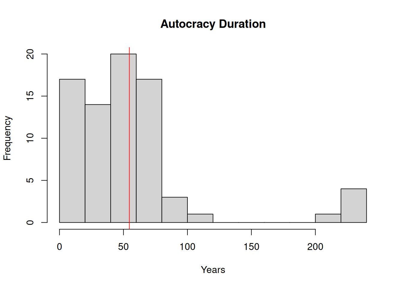
hist(
  democracy_2020[democracy_2020$democracy == 1,]$democracy_duration,
  main = "Democracy Duration", xlab = "Years"
)
abline(v = mean_duration_democracy, col = "red")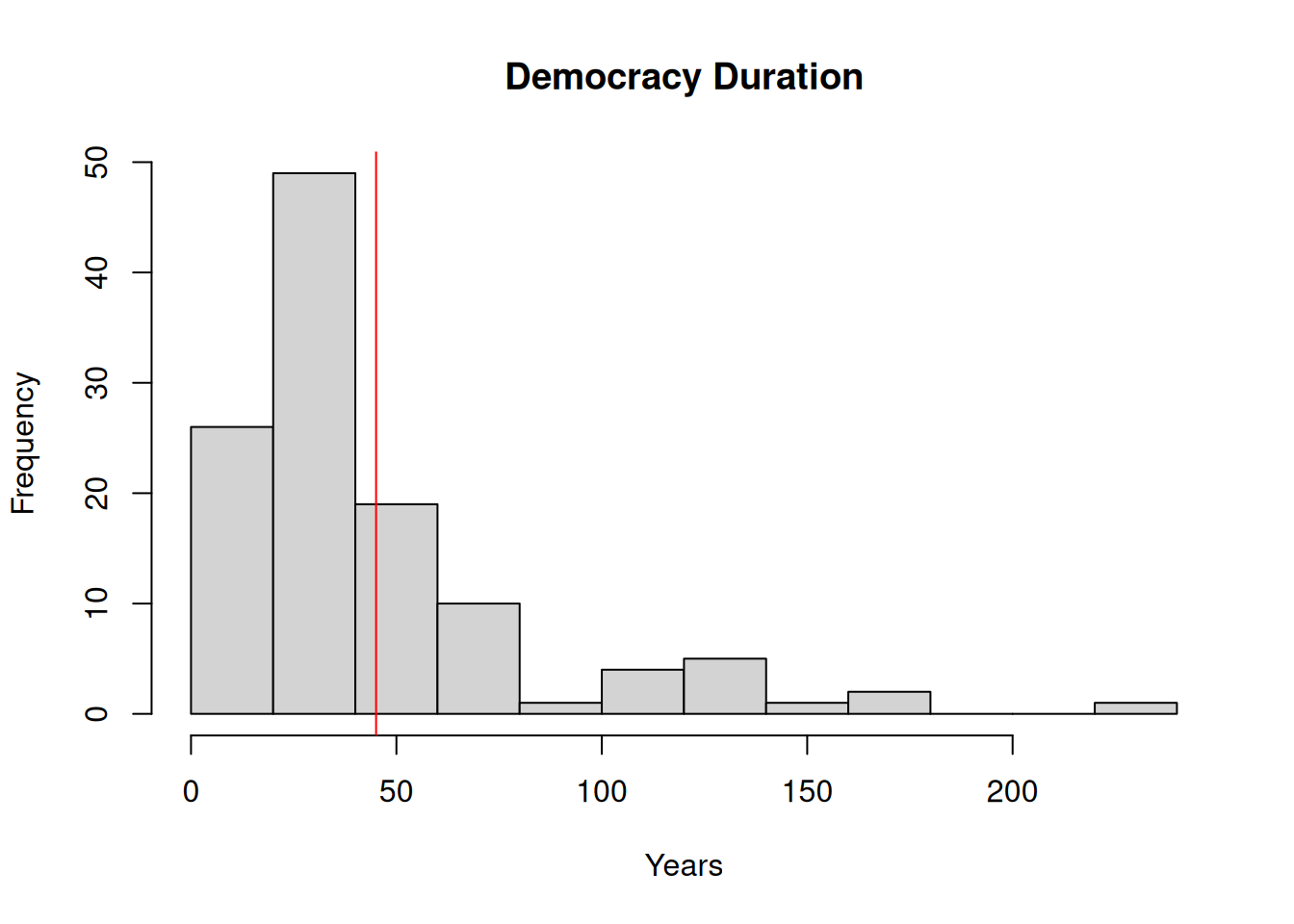
Before proceeding with formal statistical test let’s check what it the difference in means:
mean_duration_autocracy - mean_duration_democracy[1] 9.559542We can also use R for calculating quantities that can be used for conducting the test manually as we looked at in the lecture.
nrow(democracy_2020[democracy_2020$democracy == 0,])[1] 77var(democracy_2020[democracy_2020$democracy == 0,]$democracy_duration)[1] 2498.004nrow(democracy_2020[democracy_2020$democracy == 1,])[1] 118var(democracy_2020[democracy_2020$democracy == 1,]$democracy_duration)[1] 1521.604Now we could use these quantities for calculating a t test statistic like this:
\[ \begin{aligned} t = \frac{\bar{Y}_{X = 0} - \bar{Y}_{X = 1}}{\sqrt{\frac{s^2_{X = 0}}{n_{X = 0}} + \frac{s^2_{X = 1}}{n_{X = 1}}}} = \\ \frac{54.61 - 45.05}{\sqrt{\frac{2498.004}{77} + \frac{1521.604}{118}}} = \\ \frac{9.56}{6.73} \approx \\ 1.42 \end{aligned} \]
As the number of observations is more than 30 we can use already familiar pnorm() function for calculating probability density from a standard normal distribution that corresponds to this value of the test statistic (rather than using pt() function that does the same for t distribution). Since we are conducting a two-tail test (of no difference) we need to multiply our p-value by 2:
(1 - pnorm(1.42)) * 2[1] 0.1556077Now instead of doing this test step-by-step let R do all the work for us!
t.test(democracy_2020$democracy_duration ~ democracy_2020$democracy)
    Welch Two Sample t-test

data:  democracy_2020$democracy_duration by democracy_2020$democracy
t = 1.4198, df = 134.61, p-value = 0.158
alternative hypothesis: true difference in means between group 0 and group 1 is not equal to 0
95 percent confidence interval:
 -3.75709 22.87617
sample estimates:
mean in group 0 mean in group 1
       54.61039        45.05085
What do these numbers tell you? What is a null hypothesis and an alternative hypothesis for this test? What is your decision regarding a null hypothesis given the output above?