Week 6: Correlation

POP88162 Introduction to Quantitative Research Methods

Scatterplot

Let’s start by looking at the scatterplot showing the joint distribution of regime longevity and GDP per capita in 2020.

Download and read in the CSV file containing the data for these two variables called democracy_gdp_2020.csv. Remember, you will need to change the file path to the one that is correct for your computer.

democracy_gdp_2020 <- read.csv("../data/democracy_gdp_2020.csv")

As we covered in the lecture, scatterplot is the easiest way to show how two interval-scale variables relate to each other. We already used plot() function before.

plot(democracy_gdp_2020$democracy_duration, democracy_gdp_2020$gdp_per_capita)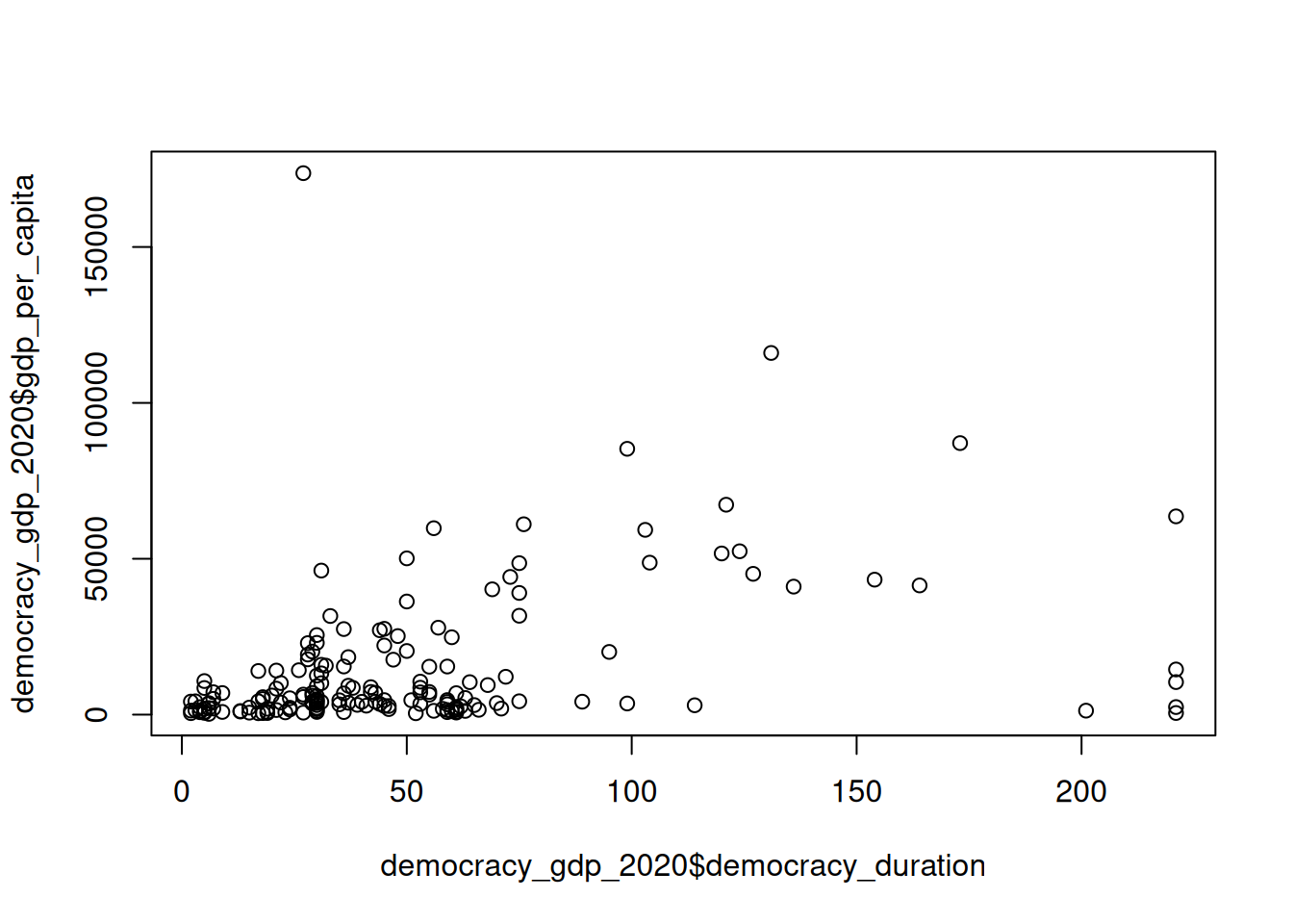

Let’s colour individual observations by their associated regime type:

plot(
  democracy_gdp_2020$democracy_duration,
  democracy_gdp_2020$gdp_per_capita,
  col = democracy_gdp_2020$democracy + 1
)

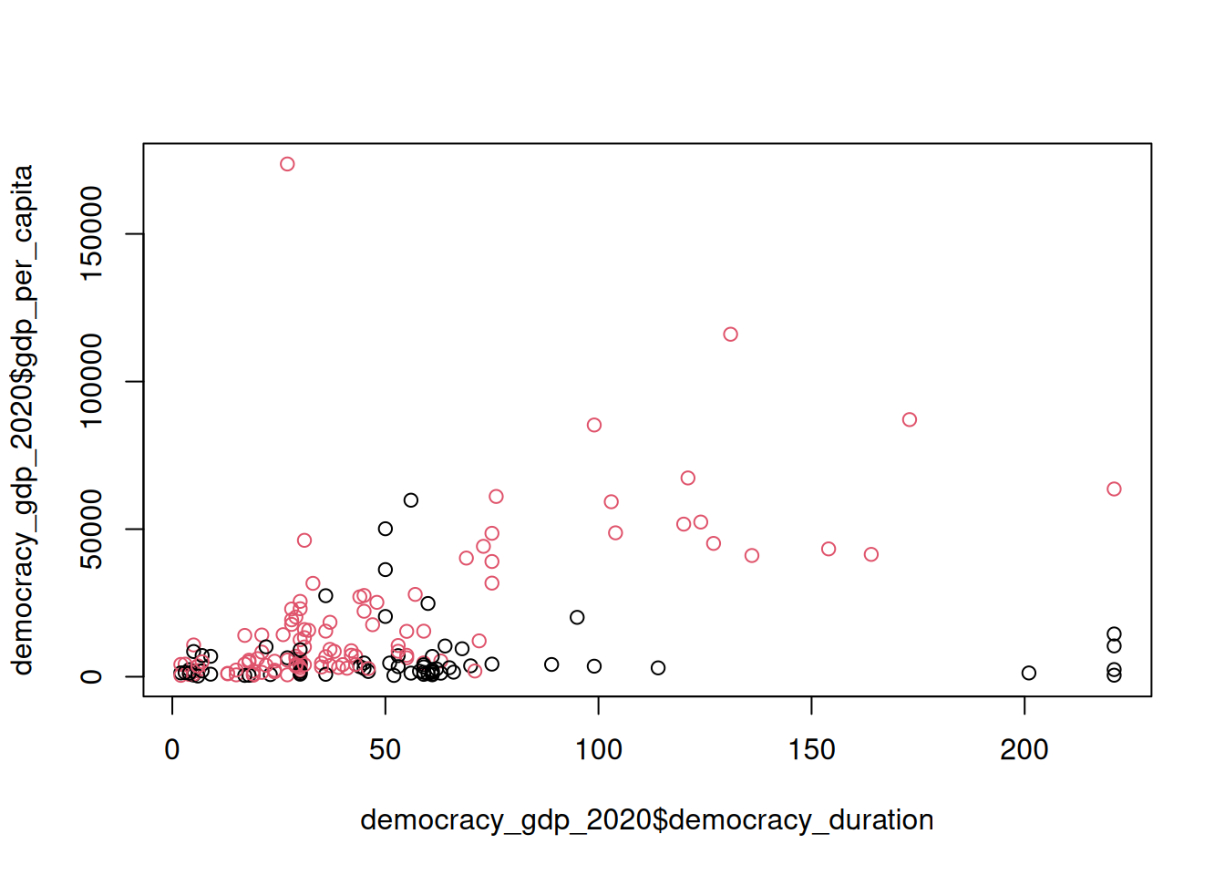
We are adding \(1\) here to avoid white colour which would be the default for \(0\) values that in our context is just how a specific level (‘autocracies’) of binary categorical variable democracy is coded.

Log Transformation

Log transformation is a widely-used approach to working with highly-skewed data. As we saw in the lecture, a distribution of a variable transformed using natural logarithm with log() function looks a lot more like normal than the original.

Compare the two histograms for GDP per capita variable below:

hist(democracy_gdp_2020$gdp_per_capita)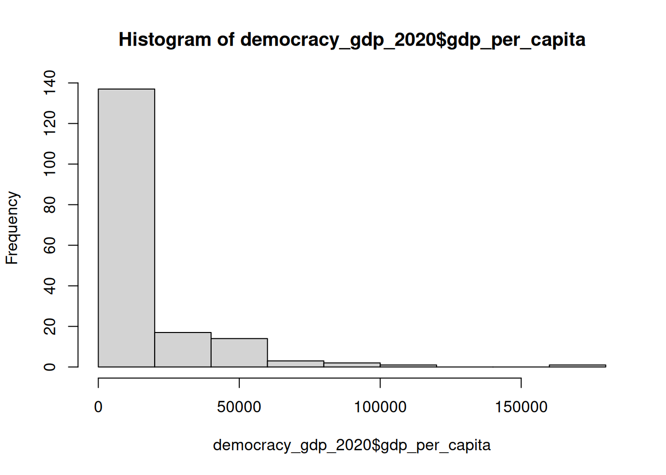

hist(log(democracy_gdp_2020$gdp_per_capita))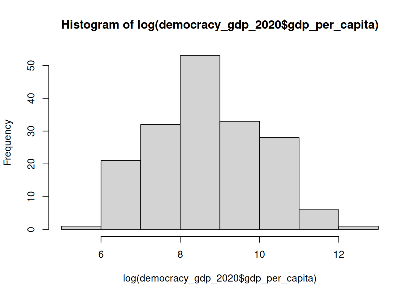

Calculate the mean for each of the two (original and log-transformed) distributions and add those to the histogram using abline() function. If you are unsure about the arguments needed you can always check the help file by adding a question mark ? before the function name like this: ?abline.

Now re-do the scatterplot from above, where each variable is log transformed.

Correlation

Calculate Pearson correlation coefficient between the two variables using cor() function.

What are its direction and magnitude?

Now carry out a statistical test using cor.test() function.

What do these numbers tell you? What is a null hypothesis and an alternative hypothesis for this test? What is your decision regarding a null hypothesis given the output above?