democracy_gdp_2020 <- read.csv("../data/democracy_gdp_2020.csv")Week 12: Logistic Regression
POP88162 Introduction to Quantitative Research Methods
Plotting
Read in the data democracy_gdp_2020.csv. Use the file provided for this week as it contains additional variable representing former colonial status. You can find this dataset on Blackboard.
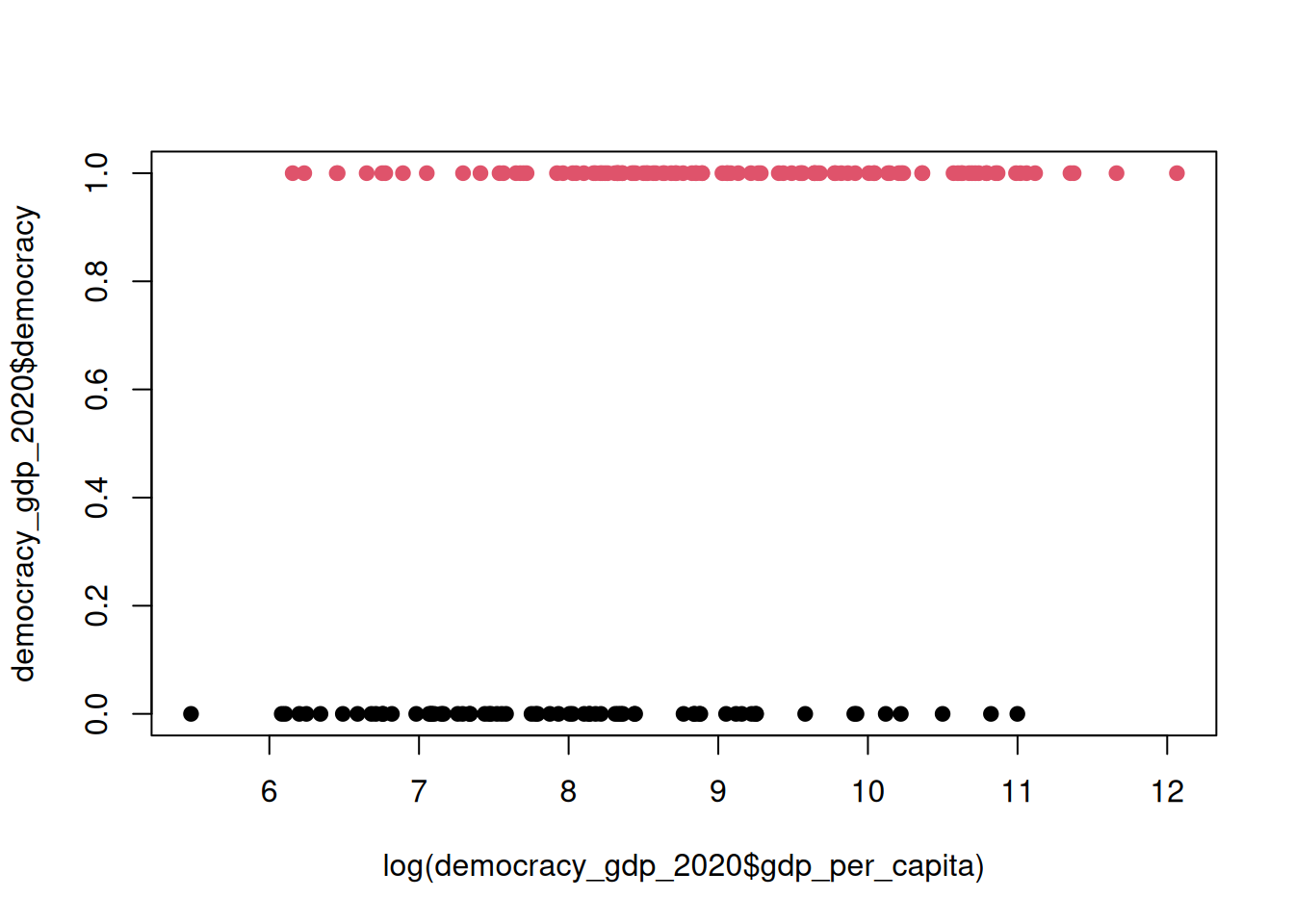
Let’s start by replicating the plot with continuous independent and binary dependent variable.
plot(
  log(democracy_gdp_2020$gdp_per_capita), # X
  democracy_gdp_2020$democracy, # Y
  pch = 19, # Type of point
  col = democracy_gdp_2020$democracy + 1 # Add 1 to avoid white colour
)
Linear Probability Model
Start by fitting a linear probability model to the data, with binary indicator for democracy as the dependent variable and log GDP per capita as independent variable. We use lm() function here as this model is, essentially, just a linear regression model with a binary dependent variable.
lpm_fit <- lm(democracy ~ log(gdp_per_capita), data = democracy_gdp_2020)
summary(lpm_fit)
Call:
lm(formula = democracy ~ log(gdp_per_capita), data = democracy_gdp_2020)

Residuals:
    Min      1Q  Median      3Q     Max
-0.9363 -0.4372  0.1502  0.3861  0.7243

Coefficients:
                    Estimate Std. Error t value Pr(>|t|)
(Intercept)         -0.56415    0.21644  -2.606  0.00995 **
log(gdp_per_capita)  0.13642    0.02468   5.527 1.18e-07 ***
---
Signif. codes:  0 '***' 0.001 '**' 0.01 '*' 0.05 '.' 0.1 ' ' 1

Residual standard error: 0.4507 on 173 degrees of freedom
  (20 observations deleted due to missingness)
Multiple R-squared:  0.1501,    Adjusted R-squared:  0.1452
F-statistic: 30.54 on 1 and 173 DF,  p-value: 1.183e-07
What do these numbers tell you? What is your substantive interpertation of the estimates?
Now re-fit this model using fomer colonial status (variable noncol) as another independent variable. How did your estimates change?
Let’s add the fitter linear regression line to our scatterplot.
plot(
  log(democracy_gdp_2020$gdp_per_capita), # X
  democracy_gdp_2020$democracy, # Y
  xlim = c(log(50), log(1000000)), # Expand x-axis to better see how LPM behaves at the edges
  pch = 19,
  col = democracy_gdp_2020$democracy + 1
)
abline(lpm_fit, col = "red")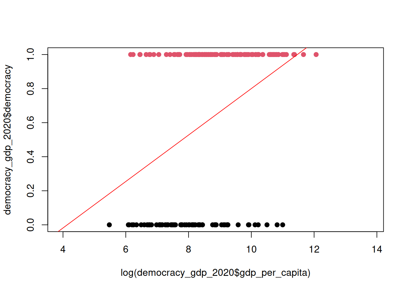
Logistic Regression Model
Now let’s fit a logistic regression model to the same data. Instead of using lm() function we will be using glm() (for generalized linear model) function. Note that in order to fit a logit model we need to specify family argument. The default value results in glm() fitting a linear model equivalent to the one that one could be fit using lm().
glm_fit <- glm( # Note that we use glm() funtion rather than lm()
  democracy ~ log(gdp_per_capita) + noncol,
  family = binomial(link = "logit"), # tells R to use logit
  data = democracy_gdp_2020
)
How would you interpret the resultant coefficients? What is a null hypothesis and an alternative hypothesis for this test? What is your decision regarding a null hypothesis given the output above?