Exploratory data analysis
- "Exploratory data analysis can never be the whole story, but nothing else can serve as the foundation stone--as the first step." (Tukey, 1977)
- Exploratory data analysis (EDA) is the first and often most important step in research
- Study's feasibility, scope and framing would usually depend on its results
- Specific details of EDA depend upon the type and quality of data available
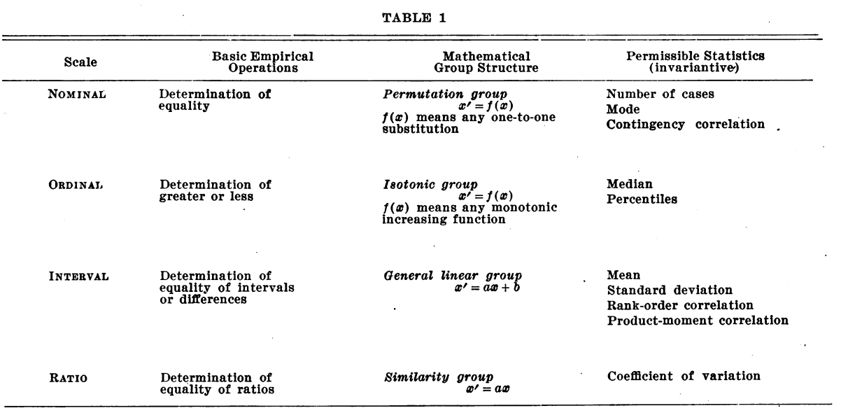
Measurement scales in Pandas
- The 4 measurement scales defined by Stevens (1946) can be roughly represented in pandas as follows:
- Interval and ratio -> numeric
- Nominal and ordinal -> categorical
Loading the dataset
In [1]:
import pandas as pd
In [2]:
# This time let's skip the 2nd row, which contains questions
kaggle2021 = pd.read_csv('../data/kaggle_survey_2021_responses.csv', skiprows = [1])
kaggle2021.head(n = 1)
/tmp/ipykernel_20081/2302513793.py:2: DtypeWarning: Columns (195,201) have mixed types. Specify dtype option on import or set low_memory=False.
  kaggle2021 = pd.read_csv('../data/kaggle_survey_2021_responses.csv', skiprows = [1])
Out[2]:
| Time from Start to Finish (seconds) | Q1 | Q2 | Q3 | Q4 | Q5 | Q6 | Q7_Part_1 | Q7_Part_2 | Q7_Part_3 | ... | Q38_B_Part_3 | Q38_B_Part_4 | Q38_B_Part_5 | Q38_B_Part_6 | Q38_B_Part_7 | Q38_B_Part_8 | Q38_B_Part_9 | Q38_B_Part_10 | Q38_B_Part_11 | Q38_B_OTHER | |
|---|---|---|---|---|---|---|---|---|---|---|---|---|---|---|---|---|---|---|---|---|---|
| 0 | 910 | 50-54 | Man | India | Bachelor’s degree | Other | 5-10 years | Python | R | NaN | ... | NaN | NaN | NaN | NaN | NaN | NaN | NaN | NaN | NaN | NaN |
1 rows × 369 columns
In [3]:
# We will load the questions as a separate dataset
kaggle2021_qs = pd.read_csv('../data/kaggle_survey_2021_responses.csv', nrows = 1)
kaggle2021_qs
Out[3]:
| Time from Start to Finish (seconds) | Q1 | Q2 | Q3 | Q4 | Q5 | Q6 | Q7_Part_1 | Q7_Part_2 | Q7_Part_3 | ... | Q38_B_Part_3 | Q38_B_Part_4 | Q38_B_Part_5 | Q38_B_Part_6 | Q38_B_Part_7 | Q38_B_Part_8 | Q38_B_Part_9 | Q38_B_Part_10 | Q38_B_Part_11 | Q38_B_OTHER | |
|---|---|---|---|---|---|---|---|---|---|---|---|---|---|---|---|---|---|---|---|---|---|
| 0 | Duration (in seconds) | What is your age (# years)? | What is your gender? - Selected Choice | In which country do you currently reside? | What is the highest level of formal education ... | Select the title most similar to your current ... | For how many years have you been writing code ... | What programming languages do you use on a reg... | What programming languages do you use on a reg... | What programming languages do you use on a reg... | ... | In the next 2 years, do you hope to become mor... | In the next 2 years, do you hope to become mor... | In the next 2 years, do you hope to become mor... | In the next 2 years, do you hope to become mor... | In the next 2 years, do you hope to become mor... | In the next 2 years, do you hope to become mor... | In the next 2 years, do you hope to become mor... | In the next 2 years, do you hope to become mor... | In the next 2 years, do you hope to become mor... | In the next 2 years, do you hope to become mor... |
1 rows × 369 columns
Summarizing numeric variables
- DataFrame methods in pandas can automatically handle (exclude) missing data (
NaN)
In [4]:
kaggle2021.describe() # DataFrame.describe() provides an range of summary statistics
Out[4]:
| Time from Start to Finish (seconds) | Q30_B_Part_1 | Q30_B_Part_2 | Q30_B_Part_3 | Q30_B_Part_4 | Q30_B_Part_5 | Q30_B_Part_6 | Q30_B_Part_7 | Q30_B_OTHER | |
|---|---|---|---|---|---|---|---|---|---|
| count | 2.597300e+04 | 0.0 | 0.0 | 0.0 | 0.0 | 0.0 | 0.0 | 0.0 | 0.0 |
| mean | 1.105466e+04 | NaN | NaN | NaN | NaN | NaN | NaN | NaN | NaN |
| std | 1.014716e+05 | NaN | NaN | NaN | NaN | NaN | NaN | NaN | NaN |
| min | 1.200000e+02 | NaN | NaN | NaN | NaN | NaN | NaN | NaN | NaN |
| 25% | 4.430000e+02 | NaN | NaN | NaN | NaN | NaN | NaN | NaN | NaN |
| 50% | 6.560000e+02 | NaN | NaN | NaN | NaN | NaN | NaN | NaN | NaN |
| 75% | 1.038000e+03 | NaN | NaN | NaN | NaN | NaN | NaN | NaN | NaN |
| max | 2.488653e+06 | NaN | NaN | NaN | NaN | NaN | NaN | NaN | NaN |
Methods for summarizing numeric variables
In [5]:
kaggle2021.iloc[:,0].mean() # Rather than using describe(), we can apply individual methods
Out[5]:
11054.66492126439
In [6]:
kaggle2021.iloc[:,0].median() # Median
Out[6]:
656.0
In [7]:
kaggle2021.iloc[:,0].std() # Standard deviation
Out[7]:
101471.6221245172
In [8]:
import statistics ## We don't have to rely only on methods provided by `pandas`
statistics.stdev(kaggle2021.iloc[:,0])
Out[8]:
101471.6221245172
Summarizing categorical variables
In [9]:
kaggle2021.describe(include = 'all') # Adding include = 'all' tells pandas to summarize all variables
Out[9]:
| Time from Start to Finish (seconds) | Q1 | Q2 | Q3 | Q4 | Q5 | Q6 | Q7_Part_1 | Q7_Part_2 | Q7_Part_3 | ... | Q38_B_Part_3 | Q38_B_Part_4 | Q38_B_Part_5 | Q38_B_Part_6 | Q38_B_Part_7 | Q38_B_Part_8 | Q38_B_Part_9 | Q38_B_Part_10 | Q38_B_Part_11 | Q38_B_OTHER | |
|---|---|---|---|---|---|---|---|---|---|---|---|---|---|---|---|---|---|---|---|---|---|
| count | 2.597300e+04 | 25973 | 25973 | 25973 | 25973 | 25973 | 25973 | 21860 | 5334 | 10756 | ... | 633 | 591 | 4239 | 729 | 737 | 1020 | 666 | 2747 | 4542 | 377 |
| unique | NaN | 11 | 5 | 66 | 7 | 15 | 7 | 1 | 1 | 1 | ... | 1 | 1 | 1 | 1 | 1 | 1 | 1 | 1 | 1 | 1 |
| top | NaN | 25-29 | Man | India | Master’s degree | Student | 1-3 years | Python | R | SQL | ... | Comet.ml | Sacred + Omniboard | TensorBoard | Guild.ai | Polyaxon | ClearML | Domino Model Monitor | MLflow | None | Other |
| freq | NaN | 4931 | 20598 | 7434 | 10132 | 6804 | 7874 | 21860 | 5334 | 10756 | ... | 633 | 591 | 4239 | 729 | 737 | 1020 | 666 | 2747 | 4542 | 377 |
| mean | 1.105466e+04 | NaN | NaN | NaN | NaN | NaN | NaN | NaN | NaN | NaN | ... | NaN | NaN | NaN | NaN | NaN | NaN | NaN | NaN | NaN | NaN |
| std | 1.014716e+05 | NaN | NaN | NaN | NaN | NaN | NaN | NaN | NaN | NaN | ... | NaN | NaN | NaN | NaN | NaN | NaN | NaN | NaN | NaN | NaN |
| min | 1.200000e+02 | NaN | NaN | NaN | NaN | NaN | NaN | NaN | NaN | NaN | ... | NaN | NaN | NaN | NaN | NaN | NaN | NaN | NaN | NaN | NaN |
| 25% | 4.430000e+02 | NaN | NaN | NaN | NaN | NaN | NaN | NaN | NaN | NaN | ... | NaN | NaN | NaN | NaN | NaN | NaN | NaN | NaN | NaN | NaN |
| 50% | 6.560000e+02 | NaN | NaN | NaN | NaN | NaN | NaN | NaN | NaN | NaN | ... | NaN | NaN | NaN | NaN | NaN | NaN | NaN | NaN | NaN | NaN |
| 75% | 1.038000e+03 | NaN | NaN | NaN | NaN | NaN | NaN | NaN | NaN | NaN | ... | NaN | NaN | NaN | NaN | NaN | NaN | NaN | NaN | NaN | NaN |
| max | 2.488653e+06 | NaN | NaN | NaN | NaN | NaN | NaN | NaN | NaN | NaN | ... | NaN | NaN | NaN | NaN | NaN | NaN | NaN | NaN | NaN | NaN |
11 rows × 369 columns
Methods for summarizing categorical variables
In [10]:
kaggle2021.iloc[:,2].mode() # Mode, most frequent value
Out[10]:
0    Man
Name: Q2, dtype: object
In [11]:
kaggle2021.iloc[:,2].value_counts() # Counts of unique values
Out[11]:
Man                        20598
Woman                       4890
Prefer not to say            355
Nonbinary                     88
Prefer to self-describe       42
Name: Q2, dtype: int64
In [12]:
kaggle2021.iloc[:,2].value_counts(normalize = True) # We can further normalize them by the number of rows
Out[12]:
Man                        0.793054
Woman                      0.188272
Prefer not to say          0.013668
Nonbinary                  0.003388
Prefer to self-describe    0.001617
Name: Q2, dtype: float64
Summary of descriptive statistics methods
| Method | Numeric | Categorical | Description |
|---|---|---|---|
count |
yes | yes | Number of non-NA observations |
value_counts |
yes | yes | Number of unique observations by value |
describe |
yes | yes | Set of summary statistics for Series/DataFrame |
min, max |
yes | yes (caution) | Minimum and maximum values |
quantile |
yes | no | Sample quantile ranging from 0 to 1 |
sum |
yes | yes (caution) | Sum of values |
prod |
yes | no | Product of values |
mean |
yes | no | Mean |
median |
yes | no | Median (50% quantile) |
var |
yes | no | Sample variance |
std |
yes | no | Sample standard deviation |
skew |
yes | no | Sample skewness (third moment) |
kurt |
yes | no | Sample kurtosis (fourth moment) |
Crosstabulation
- When working with survey data it is often useful to perform simple crosstabulations
- Crosstabulation (or crosstab for short) is a computation of group frequencies
- It is usually used for working with categorical variables that have a limited number of categories
- In pandas
pd.crosstab()method is a special case ofpd.pivot_table()
Crosstabulation in pandas
In [13]:
# Calculate crosstabulation between 'Age group' (Q1) and 'Gender' (Q2)
pd.crosstab(kaggle2021['Q1'], kaggle2021['Q2'])
Out[13]:
| Q2 | Man | Nonbinary | Prefer not to say | Prefer to self-describe | Woman |
|---|---|---|---|---|---|
| Q1 | |||||
| 18-21 | 3696 | 16 | 60 | 12 | 1117 |
| 22-24 | 3643 | 13 | 66 | 9 | 963 |
| 25-29 | 3859 | 12 | 61 | 5 | 994 |
| 30-34 | 2765 | 17 | 34 | 7 | 618 |
| 35-39 | 1993 | 7 | 42 | 7 | 455 |
| 40-44 | 1537 | 4 | 31 | 1 | 317 |
| 45-49 | 1171 | 4 | 24 | 1 | 175 |
| 50-54 | 811 | 3 | 14 | 0 | 136 |
| 55-59 | 509 | 4 | 7 | 0 | 72 |
| 60-69 | 504 | 4 | 10 | 0 | 35 |
| 70+ | 110 | 4 | 6 | 0 | 8 |
Margins in crosstab
In [14]:
# It is often useful to see the proportions/percentages rather than raw counts
pd.crosstab(kaggle2021['Q1'], kaggle2021['Q2'], normalize = 'columns')
Out[14]:
| Q2 | Man | Nonbinary | Prefer not to say | Prefer to self-describe | Woman |
|---|---|---|---|---|---|
| Q1 | |||||
| 18-21 | 0.179435 | 0.181818 | 0.169014 | 0.285714 | 0.228425 |
| 22-24 | 0.176862 | 0.147727 | 0.185915 | 0.214286 | 0.196933 |
| 25-29 | 0.187348 | 0.136364 | 0.171831 | 0.119048 | 0.203272 |
| 30-34 | 0.134236 | 0.193182 | 0.095775 | 0.166667 | 0.126380 |
| 35-39 | 0.096757 | 0.079545 | 0.118310 | 0.166667 | 0.093047 |
| 40-44 | 0.074619 | 0.045455 | 0.087324 | 0.023810 | 0.064826 |
| 45-49 | 0.056850 | 0.045455 | 0.067606 | 0.023810 | 0.035787 |
| 50-54 | 0.039373 | 0.034091 | 0.039437 | 0.000000 | 0.027812 |
| 55-59 | 0.024711 | 0.045455 | 0.019718 | 0.000000 | 0.014724 |
| 60-69 | 0.024468 | 0.045455 | 0.028169 | 0.000000 | 0.007157 |
| 70+ | 0.005340 | 0.045455 | 0.016901 | 0.000000 | 0.001636 |
Crosstabulation in pandas with pivot_table
In [15]:
# For `values` variable we use `Q3`, but any other would work equally well
pd.pivot_table(kaggle2021, index = 'Q1', columns = 'Q2', values = 'Q3', aggfunc = 'count', fill_value = 0)
Out[15]:
| Q2 | Man | Nonbinary | Prefer not to say | Prefer to self-describe | Woman |
|---|---|---|---|---|---|
| Q1 | |||||
| 18-21 | 3696 | 16 | 60 | 12 | 1117 |
| 22-24 | 3643 | 13 | 66 | 9 | 963 |
| 25-29 | 3859 | 12 | 61 | 5 | 994 |
| 30-34 | 2765 | 17 | 34 | 7 | 618 |
| 35-39 | 1993 | 7 | 42 | 7 | 455 |
| 40-44 | 1537 | 4 | 31 | 1 | 317 |
| 45-49 | 1171 | 4 | 24 | 1 | 175 |
| 50-54 | 811 | 3 | 14 | 0 | 136 |
| 55-59 | 509 | 4 | 7 | 0 | 72 |
| 60-69 | 504 | 4 | 10 | 0 | 35 |
| 70+ | 110 | 4 | 6 | 0 | 8 |
Data visualization in Python
- As with dealing with data, Python has no in-built, 'base' plotting functionality
matplotlibhas become the one of standard solutions- It is often used in combination with
pandas - Other popular alternative include
seabornandplotnine - Also
pandasitself has some limited plotting facilities
plotnine - ggplot for Python
plotnineimplements Grammar of Graphics data visualisation scheme (Wilkinson, 2005)- It mimics the syntax of a well-known R library
ggplot2syntax (Wickham, 2010) - In doing so, it makes the code (almost) seamlessly portable between the two languages
Grammar of graphics
- Grammar of Graphics is a powerful conceptualization of plotting
- Graphs are broken into multiple layers
- Layers can be recycled across multiple plots
Structure of ggplot calls in plotnine
- Creation of ggplot objects in
plotlinehas the following structure:
ggplot(data = <DATA>) +\
<GEOM_FUNCTION>(mapping = aes(<MAPPINGS>))- If the mappings are re-used across geometric objects (e.g. scatterplot and line):
ggplot(data = <DATA>, mapping = aes(<MAPPINGS>)) +\
    <GEOM_FUNCTION>() +\
    <GEOM_FUNCTION>()
Creating a ggplot in plotnine
In [16]:
from plotnine import *
In [17]:
q1_plot = ggplot(data = kaggle2021) + geom_bar(aes(x = 'Q1')) # Basic 'Age group' (Q1) bar chart
q1_plot

Out[17]:
<ggplot: (8783323507023)>
Compare to base pandas
In [24]:
# First we need to group dataset by 'Age group' (Q1) and summarize it with `size()`
kaggle2021_q1_grouped = kaggle2021.groupby(['Q1']).size()
kaggle2021_q1_grouped.head(n = 3)
Out[24]:
Q1
18-21    4901
22-24    4694
25-29    4931
dtype: int64
In [19]:
kaggle2021_q1_grouped.plot(kind = 'bar')
Out[19]:
<AxesSubplot:xlabel='Q1'>

Compare to matplotlib
In [20]:
import matplotlib.pyplot as plt
In [21]:
# `matplotlib` is more low-level library
# plots would need more work to be 'prettified'
plt.bar(x = kaggle2021_q1_grouped.index, height = kaggle2021_q1_grouped.values)
Out[21]:
<BarContainer object of 11 artists>

Prettifying ggplot in plotnine
In [22]:
# Here we change default axes' labels and then apply B&W theme
q1_plot_pretty = q1_plot +\
    labs(x = 'Age group', y = 'respondents') +\
    theme_bw()
q1_plot_pretty

Out[22]:
<ggplot: (8783321248031)>
Other geometric objects (geom_)
| Method | Description |
|---|---|
geom_bar(), geom_col() |
Bar charts |
geom_boxplot() |
Box and whisker plot |
geom_histogram() |
Histogram |
geom_point() |
Scatterplot |
geom_line(), geom_path() |
Lines |
geom_map() |
Geographic areas |
geom_smooth() |
Smoothed conditional means |
geom_violin() |
Violin plots |
Writing plots out in plotnine
- Output format is automatically determined from write-out file extension
- Commonly used formats are PDF, PNG and EPS
In [23]:
q1_plot_pretty.save('../temp/q1_plot_pretty.pdf')
/home/tpaskhalis/Decrypted/Git/RECSM/venv/lib/python3.8/site-packages/plotnine/ggplot.py:719: PlotnineWarning: Saving 6.4 x 4.8 in image.
/home/tpaskhalis/Decrypted/Git/RECSM/venv/lib/python3.8/site-packages/plotnine/ggplot.py:722: PlotnineWarning: Filename: ../temp/q1_plot_pretty.pdf
Additional visualization materials
Books:
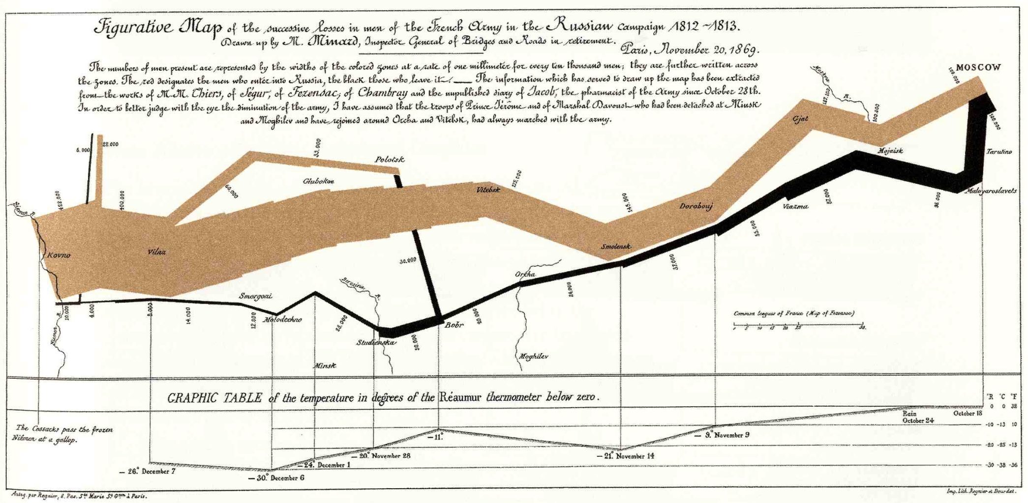
- Hieran, Kiely. 2019. Data Visualization: A Practical Introduction. Princeton, NJ: Princeton University Press
- Tufte, Edward. 2001. The Visual Display of Quantitative Information. 2nd ed. Cheshire, CT: Graphics Press
Online:
Next
- Linear regression
- Communicating results